9 Vision Transformer
Where Part 1 has been heading
Every previous chapter has introduced a new architectural primitive and proved its backward pass. Each one slotted into the VerifiedNetSpec type and earned its own hasVJP theorem, and that includes convolution, BatchNorm, residual, depthwise, SE, LayerNorm and GELU. This chapter does the same for attention, but it also does something larger: it composes every layer the framework has proved so far into one machine-checked backward pass over a complete state-of-the-art image classifier.
The destination is Theorem 154 at the end of the chapter. It says: the whole ViT-Tiny’s hand-written input-gradient chain — through the patch embedding, twelve transformer blocks with their own parameters, final LayerNorm and head, each slot the certified backward of its op at its own saved activation — equals the network’s Jacobian transpose at every input, assuming only \(\varepsilon {\gt} 0\) at the LayerNorms. The proof composes everything this chapter introduces, plus most of what the previous chapters introduced, into a tower of vjpMatComp applications with vjpComp at the joins. Read the proof’s dependency list and you see a tour of Part 1: dense, residual, layer norm, GELU, softmax, matrix multiply, plus the fourteen matrix-machinery lemmas this chapter sets up. None of them is new in its own right. What’s new is how high the composition rule can be pushed.
9.1 Run it first
Before any of the attention mathematics, train the network that needs it. Four commands, and the last network in Part 1 is also the quickest one in it:
lake exe cache get                         # Mathlib oleans, ~30 s
./scripts/datasets/download_imagenette.sh  # 330 MB dl, 2.4 GB unpacked
lake build vit-verified-adam
./.lake/build/bin/vit-verified-adam data
On one RTX 4060 Ti (CUDA 12.9), from runs/2026-08-12-vit-imagenette-xla-cuda/. XLA’s startup banner is removed, the network description line is wrapped, the per-step lines are dropped, and the middle of the run is elided:
[pjrt_ffi] XLA backend: PJRT 0.112, 1 device(s)
[pjrt_ffi] compiled verified_mlir/vit_adam_train_step.mlir
             (@vit_adam_train_step, 603 outputs, 1 replica)
             in 6104 ms
[pjrt_ffi] compiled verified_mlir/vit_fwd.mlir
             (@vit_fwd, 1 outputs, 1 replica) in 1644 ms
ViT-Tiny on Imagenette 224² (patch-16 → CLS+pos → 12 transformer
  blocks @ dim192/3heads/MLP768 → final LN → CLS-head 10)
  via the VERIFIED renderer → XLA/PJRT → GPU
  train 9469, val 3925; bs 32, ViT-Tiny adam
    (cosine+warmup 5ep, baseLR 0.000300), He init
[pjrt_ffi] RESIDENT: @vit_adam_train_step holds 600 parameter
             tensors (63.2 MB) on 1 device; they stop crossing PCIe
             from here
Epoch 1/80: loss=2.127541 lr=0.000060
  epoch 1: val_acc = 1381/3925 = 35.184713%  top5 = 3121/3925 = 79.515924%
Epoch 2/80: loss=1.869707 lr=0.000120
  epoch 2: val_acc = 1619/3925 = 41.248408%  top5 = 3350/3925 = 85.350318%
Epoch 3/80: loss=1.750333 lr=0.000180
  epoch 3: val_acc = 1591/3925 = 40.535032%  top5 = 3362/3925 = 85.656051%
Epoch 30/80: loss=1.004060 lr=0.000225
  epoch 30: val_acc = 2571/3925 = 65.503185%  top5 = 3698/3925 = 94.216561%
Epoch 79/80: loss=0.515797 lr=0.000000
  epoch 79: val_acc = 2698/3925 = 68.738854%  top5 = 3551/3925 = 90.471338%
Epoch 80/80: loss=0.515159 lr=0.000000
  epoch 80: val_acc = 2698/3925 = 68.738854%  top5 = 3549/3925 = 90.420382%
done (trained ViT-Tiny adam + cosine/warmup via packed threading).
Eighty epochs at about 18 seconds each, twenty-four minutes in total, and 68.74% top-1 with 90.42% top-5 on Imagenette’s 3,925-image validation split. The best epoch reached \(68.92\% \). That is the fastest network in this book’s Imagenette column by a wide margin and also the least accurate one in it (§9.3).
Attention in one equation
A transformer encoder block does two things to its input sequence \(X \in \mathbb {R}^{N \times d}\) (think of \(N\) image patches, each represented as a \(d\)-vector):
Multi-head self-attention (MHSA): each output row is a weighted average of all input rows, where the weights are computed from the input itself.
Per-token MLP: a small two-layer MLP applied independently to every row.
Both halves are wrapped in a LayerNorm + residual sandwich (exactly the same template as ConvNeXt’s blocks from Chapter 8, and the layout that transferred to convnets in 2022 actually came from transformers in 2017).
The interesting half is the first one. Scaled dot-product attention computes, for queries \(Q\), keys \(K\), and values \(V\) (all linear projections of \(X\)):
In words: every row of \(Q\) is compared to every row of \(K\) via inner product (the \(QK^\top \) matrix is \(N \times N\), one entry per query-key pair). Each row of that \(N \times N\) matrix is passed through softmax to get a probability distribution over the keys (which positions to attend to). Those probabilities then weight the rows of \(V\) to produce the output. The \(1 / \sqrt{d_h}\) scaling keeps the softmax from saturating at large \(d_h\). Multi-head attention just runs several copies of this in parallel on lower-dimensional projections, concatenating the outputs.
Each token, meaning each row of \(X\), ends up looking at every other token. That’s the qualitative break from CNNs: convolutions look only at a local neighborhood, attention looks everywhere. The receptive field is global from the first layer.
Why this chapter has forty theorems
The math of attention is matrix algebra. Chapter 1’s foundation rules (chain, sum, product, identity) were stated and proved for vector functions. Before we can prove backward passes through \(Q K^\top \) and the row-wise softmax, we need the matrix-level lifts of those rules: chain rule on matrices, additive fan-in on matrices, identity on matrices, plus matrix-specific moves like transpose, matmul-with-one-factor-fixed, and scalar scale. That’s the first section of theorems below (Matrix-level machinery, thirteen theorems and a definition). Every one of them is a mechanical lift of a vector-level theorem from Chapter 1, proved via the row-projection \(\mathrm{ContinuousLinearMap}\) and the existing chain rule. Pay the cost once, reuse forever.
The second section (Attention proofs, twenty-seven theorems) applies the matrix machinery to the actual attention math. Row-wise softmax (a per-row softmax applied to the \(N \times N\) score matrix) has the well-known closed-form Jacobian \(p_j(\delta _{ij} - p_i)\), and we prove the row-wise lifting that says this holds across matrices. Scaled dot-product attention’s backward decomposes into three matmul-backward applications (one for each of \(Q\), \(K\), \(V\)) plus the row-wise softmax backward, and we prove each. Then multi-head, then the attention sublayer (with residual), then the MLP sublayer (with residual), then a single transformer block, then a \(k\)-deep transformer tower, then the ViT body, then the whole network at its real shape. Each step is one or two compositions of the previous step. The chain that started at vjpComp (Theorem 11) reaches all the way to a 5.5M-parameter image classifier here.
What’s actually proved
That’s the framework-side payoff of this chapter: every architectural piece used by any Part-1 network has a machine-checked backward. With Theorem 154 for the input gradient and Theorem 157 for the parameter gradients the trainer steps on, the sentence “the gradient computed by this trainer is the mathematically correct one” is no longer a hope or a folklore result. It is a theorem the Lean kernel verifies on every build.
The empirical-side payoff comes after the theorems, in the Example section: ViT-Tiny trained on Imagenette underperforms the ConvNets, fairly dramatically, because 9,469 training images is too small for a transformer’s lack of inductive bias. That’s informative on its own terms: the data-hungry-transformer story made concrete.
9.2 The theorems
9.2.1 Matrix-level machinery
Figure 9-1 is the dependency graph of this section.
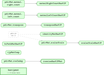
Attention is fundamentally matrix algebra: queries times keys transposed (\(QK^T\)), softmax over rows of the resulting matrix, matmul against values (\(\cdot V\)). Before we can prove backward passes through these operations, we need the matrix-level extensions of Ch 1’s foundation rules. Each theorem below is the matrix lift of a vector-level theorem from Ch 1, proved by composing the vector version with the row-projection \(\mathrm{ContinuousLinearMap}\). The Lean proofs all live in Proofs/Foundation/Tensor.lean alongside their vector counterparts. We collect them here, where the attention proofs need all of them at once.
The rank-2 analogue of Definition 10. Define \(\operatorname {pdivMat}f\, A\, (i,j)\, (k,l)\) as \(\operatorname {pdiv}\) of the row-major flattened map \(v \mapsto \mathrm{flatten}\bigl(f(\mathrm{unflatten}\, v)\bigr)\) with both index pairs encoded through the \((i, j) \leftrightarrow \text{flat}\) bijection. Then \(\mathsf{HasVJPMat}\, f\) bundles a backward function \(B\) with: for all \(A\), \(dY\), \((i, j)\),
assume:
\(g : \mathbb {R}^{n} \to \mathbb {R}^{p}\) is differentiable everywhere [h_g_diff]
prove: applying \(g\) to each row of a matrix has block-diagonal Jacobian: \(\operatorname {pdivMat}(\text{rowwise } g)\, A\, (i,j)\, (k,l) = [i = k] \cdot \operatorname {pdiv}g\, (A_i)\, j\, l\).
Coordinate factoring: the \((k, l)\) output coordinate of the flattened rowwise map is \((y \mapsto g(y)_l) \circ \mathrm{rowProj}_k\), where \(\mathrm{rowProj}_k\) is the CLM extracting row \(k\) of the flat vector.
proof: Unfold flatten/unflatten; \(\mathrm{rowProj}_k\) is a reindex, hence a CLM.Every output coordinate — hence the whole flat map — is differentiable, so \(\operatorname {fderiv}\) does not fall back to its junk default.
proof: Assumption 1 composed with the CLM of step 1; hasFDerivAt_pi assembles the coordinates’ derivatives into the whole map’s.q.e.d.
proof: Chain rule through the CLM: the derivative of \((y \mapsto g(y)_l) \circ \mathrm{rowProj}_k\) at \(\mathbf{e}_{(i,j)}\) sees \(\mathrm{rowProj}_k(\mathbf{e}_{(i,j)}) = [i = k]\, \mathbf{e}_j\), so by Definition 1 the entry is \([i = k] \cdot \operatorname {pdiv}g\, (A_i)\, j\, l\).
assume:
\(B_F\), \(B_G\) are correct backward functions (\(\mathsf{HasVJPMat}\, F\), \(\mathsf{HasVJPMat}\, G\)) [hF, hG]
the flattened forms of \(F\) and \(G\) are differentiable everywhere [hF_diff, hG_diff]
prove: \(\mathsf{HasVJPMat}\, (G \circ F)\).
Sketch: the VJP chain rule (Theorem 11) transcribed to rank-2 indices; every step is the same, with double sums where the rank-1 proof had single sums.
Define \(B(A, dY) := B_F\bigl(A,\; B_G(F(A),\, dY)\bigr)\).
suffices: \(B\) matches the \(\operatorname {pdivMat}\) contraction.
proof: Definition 117.Chain rule for \(\operatorname {pdivMat}\): \(\operatorname {pdivMat}(G \circ F)\, A\, (i,j)\, (k,l) = \sum _{p,q} \operatorname {pdivMat}F\, A\, (i,j)\, (p,q) \cdot \operatorname {pdivMat}G\, (F A)\, (p,q)\, (k,l)\).
proof: The flattened composite is the composite of the flattened maps (unflatten \(\circ \) flatten cancels), so the rank-1 chain rule (Theorem 2) applies at the flat level, applicable by assumption 2; re-index the flat middle sum to \((p, q)\) pairs.q.e.d.
proof: Expand the two correct fields in 1, substitute 3, and swap the two double sums (pack indices into pairs, Finset.sum_comm, unpack); with 2 this is the goal — step for step the proof of Theorem 11.
Rank-2 transcription of Theorem 12: given \(\mathsf{HasVJPMat}\) for \(F\) and \(G\) (with flat differentiability), \(\mathsf{HasVJPMat}\, (F + G)\) with backward \(B_F(A, dY) + B_G(A, dY)\).
suffices: the summed backward matches the \(\operatorname {pdivMat}\) contraction.
proof: Definition 117.q.e.d.
proof: Expand both correct fields, merge the double sums (Finset.sum_add_distrib twice); the sum rule for \(\operatorname {pdivMat}\) — Theorem 3 through the flatten bijection — rewrites \(\operatorname {pdivMat}F + \operatorname {pdivMat}G = \operatorname {pdivMat}(F + G)\).
\(\mathsf{HasVJPMat}\, (\mathrm{id})\), backward \(B(A, dY) = dY\).
\(\operatorname {pdivMat}(\mathrm{id})\, A\, (i,j)\, (k,l) = [i = k \wedge j = l]\).
proof: Flatten \(\circ \) unflatten is the identity on the flat vector, so the identity Jacobian (Theorem 5) applies; the flat-index equality decodes to \(i = k \wedge j = l\) by injectivity of the pairing.q.e.d.
proof: Contract 1 with \(dY\): the two-dimensional Kronecker sum collapses to \(dY_{ij}\) (simp with ite_and); Definition 117 closes.
prove: \(\operatorname {pdivMat}(M \mapsto s \cdot M)\, A\, (i,j)\, (k,l) = [i = k \wedge j = l] \cdot s\).
The flattened scalar-scale map reduces to \(v \mapsto s \cdot v\).
proof: Flatten/unflatten round-trip, pointwise.\(\operatorname {pdiv}(v \mapsto s \cdot v) = s \cdot \delta \) at the flat indices.
proof: Scalar-multiple rule (pdiv_const_smul: the product rule, Theorem 4, at a constant factor whose own Jacobian vanishes, Theorem 6), then the identity Jacobian (Theorem 5).q.e.d.
proof: The flat-index equality decodes to \(i = k \wedge j = l\) by injectivity of the pairing.
prove: \(\operatorname {pdivMat}(\mathrm{transpose})\, A\, (i,j)\, (k,l) = [j = k \wedge i = l]\).
The flattened transpose is a pure gather: at output index \(\mathrm{idx}\), it reads \(v\) at the index with components swapped.
proof: Unfold transpose/flatten/unflatten.q.e.d.
proof: Reindex Jacobian (Theorem 7) with the swap map \(\sigma \): the indicator condition \(\mathrm{flat}(i,j) = \mathrm{flat}(l,k)\) decodes to \(j = k \wedge i = l\) by injectivity of the pairing.
prove: \(\operatorname {pdivMat}(B' \mapsto C \cdot B')\, B\, (i,j)\, (k,l) = [l = j] \cdot C_{ki}\).
The flattened map \(v \mapsto \mathrm{flatten}(C \cdot \mathrm{unflatten}\, v)\) is linear: additive and homogeneous in \(v\).
proof: Unfold \(\mathrm{Mat.mul}\)/flatten/unflatten; mul_add, Finset.sum_add_distrib, Finset.mul_sum.The Jacobian entry at \((i,j) \to (k,l)\) is \((C \cdot E_{ij})_{kl}\), where \(E_{ij} = \mathrm{unflatten}(\mathbf{e}_{\mathrm{flat}(i,j)})\) is the matrix unit.
proof: Linear rule (Theorem 9 at \(c = 0\), pdiv_of_linear).q.e.d.
proof: \((C \cdot E_{ij})_{kl} = \sum _s C_{ks}\, [s = i \wedge l = j] = [l = j] \cdot C_{ki}\); case split on \(l = j\).
prove: \(\operatorname {pdivMat}(A' \mapsto A' \cdot D)\, A\, (i,j)\, (k,l) = [i = k] \cdot D_{jl}\).
Mirror image of Theorem 124: the flattened map \(v \mapsto \mathrm{flatten}(\mathrm{unflatten}\, v \cdot D)\) is linear, so by the linear rule (pdiv_of_linear) the Jacobian entry is \((E_{ij} \cdot D)_{kl} = [i = k] \cdot D_{jl}\); case split on \(i = k\).
\(\mathsf{HasVJPMat}\, (B' \mapsto C \cdot B')\), backward \(dB = C^{T} \cdot dY\).
Define \(B(B', dY)_{ij} := \sum _k C_{ki}\, dY_{kj}\) (that is, \(C^T \cdot dY\)).
suffices: \(B\) matches the \(\operatorname {pdivMat}\) contraction.
proof: Definition 117.q.e.d.
proof: Substitute the Jacobian (Theorem 124): \(\sum _{k,l} [l = j]\, C_{ki} \cdot dY_{kl}\) collapses at \(l = j\) (Finset.sum_ite_eq’) to \(\sum _k C_{ki}\, dY_{kj} = B\).
\(\mathsf{HasVJPMat}\, (A' \mapsto A' \cdot D)\), backward \(dA = dY \cdot D^{T}\).
Define \(B(A', dY)_{ij} := \sum _l dY_{il}\, D_{jl}\) (that is, \(dY \cdot D^T\)).
suffices: \(B\) matches the \(\operatorname {pdivMat}\) contraction.
proof: Definition 117.q.e.d.
proof: Substitute the Jacobian (Theorem 125): \(\sum _{k,l} [i = k]\, D_{jl} \cdot dY_{kl}\) collapses at \(k = i\) (Finset.sum_ite_eq) to \(\sum _l D_{jl}\, dY_{il} = B\).
\(\mathsf{HasVJPMat}\, (M \mapsto s \cdot M)\), backward \(dA = s \cdot dY\).
\(\mathsf{HasVJPMat}\, (\mathrm{transpose})\), backward \(dA = dY^{T}\).
assume:
\(B_g\) is a correct backward for \(g : \mathbb {R}^{n} \to \mathbb {R}^{p}\) (\(\mathsf{HasVJP}\, g\)) [hg]
\(g\) is differentiable everywhere [hg_diff]
prove: \(\mathsf{HasVJPMat}\) of the rowwise map on \(\mathbb {R}^{m \times n} \to \mathbb {R}^{m \times p}\), with backward applying \(B_g\) to each row: \(B(A, dY)_r = B_g(A_r, dY_r)\).
suffices: \(B\) matches the \(\operatorname {pdivMat}\) contraction.
proof: Definition 117.The Jacobian is block-diagonal: \(\operatorname {pdivMat}= [i = k] \cdot \operatorname {pdiv}g\, (A_i)\, j\, l\).
proof: Row-independence (Theorem 118), applicable by assumption 2.q.e.d.
proof: Contract 2 with \(dY\): the row sum collapses at \(k = i\) (Finset.sum_ite_eq); what remains is precisely \(g\)’s own correctness equation at row \(i\) (assumption 1).
9.2.2 Attention proofs
Figures 9-2 and 9-3 are the dependency graph of this section, in two halves.
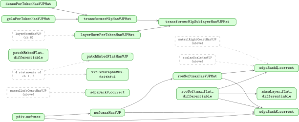
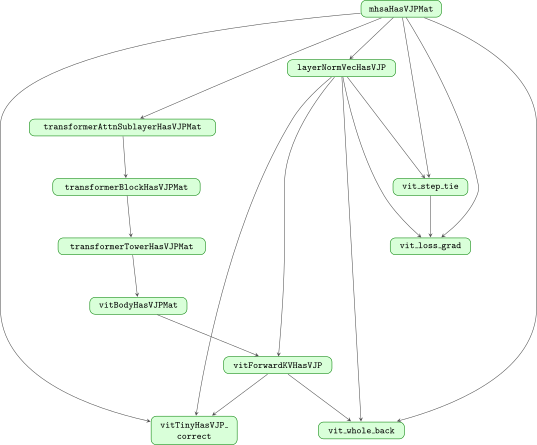
Writing \(p := \mathrm{softmax}(z)\): prove: \(\operatorname {pdiv}(\mathrm{softmax})\, z\, i\, j = p_j\, (\delta _{ij} - p_i)\).
\(\operatorname {pdiv}(\mathrm{softmax})\, z\, i\, j = \operatorname {fderiv}_{\mathbb {R}}\, \bigl(z' \mapsto e^{z'_j} \cdot (\textstyle \sum _k e^{z'_k})^{-1}\bigr)\, z\, (\mathbf{e}_i)\).
proof: Definition 1; extract the \(j\)-th coordinate (pdiv_eq_fderiv_coord), differentiable because the denominator \(S := \sum _k e^{z_k}\) is a sum of positive exponentials, hence nonzero.Differentiate the product: numerator via HasFDerivAt.exp, denominator via (hasDerivAt_inv).comp_hasFDerivAt (licensed by \(S {\gt} 0\)).
Evaluate at \(\mathbf{e}_i\): the numerator’s derivative contributes \(e^{z_j}\, \delta _{ji}\), and the denominator’s contributes \(-e^{z_j}\, S^{-2} \cdot e^{z_i}\), the inner sum collapsing by \(\sum _k e^{z_k}\, \delta _{ki} = e^{z_i}\).
q.e.d.
proof: Combine 2–3 and rewrite in terms of \(p = e^{z}/S\): \(S^{-1} e^{z_j} \delta _{ij} - e^{z_j} S^{-2} e^{z_i} = p_j(\delta _{ij} - p_i)\) (field_simp, ring).
\(\mathsf{HasVJP}\, (\mathrm{softmax})\), with the closed-form \(O(c)\) backward
where \(\langle p, dy \rangle = \sum _j p_j\, dy_j\) is one precomputed scalar — the rank-1 structure of the Jacobian is what turns the naive \(O(c^2)\) contraction into a reduction plus a broadcast, the same optimization pattern as BN and max-pool.
suffices: \(B(z, dy)_i = \sum _j \operatorname {pdiv}(\mathrm{softmax})\, z\, i\, j \cdot dy_j\).
proof: Definition 10.\(\sum _j p_j (\delta _{ij} - p_i)\, dy_j = p_i\, dy_i - p_i \sum _j p_j\, dy_j\).
proof: Substitute the softmax Jacobian (Theorem 131); split the sum, collapse the \(\delta \)-term (Finset.sum_ite_eq), factor \(p_i\) out of the second (Finset.mul_sum).q.e.d.
proof: The right side of 2 is \(p_i(dy_i - \langle p, dy\rangle ) = B(z, dy)_i\); with 1, done.
\(\mathsf{HasVJPMat}\, (\mathrm{rowSoftmax})\): rows are independent, so the backward applies the softmax backward per row.
The rowwise-lifting argument (Theorem 130) instantiated at \(g = \mathrm{softmax}\):
The Jacobian is block-diagonal with the standalone softmax Jacobian in each block.
proof: Row-independence (Theorem 118); softmax is differentiable (positive denominator).q.e.d.
proof: Contract with \(dY\), collapse the row sum at \(k = i\); what remains is Theorem 132’s correctness equation at row \(i\); Definition 117 closes.
prove: for fixed \(K, V\): \(\mathrm{sdpaBackQ}\) matches the \(\operatorname {pdivMat}\) contraction of \(Q' \mapsto \mathrm{sdpa}(Q', K, V)\).
The forward is a four-link chain:
\[ Q' \; \mapsto \; Q' K^T \; \mapsto \; \tfrac {1}{\sqrt{d}} \cdot {\mathord {@}} \; \mapsto \; \mathrm{rowSoftmax}\, {\mathord {@}} \; \mapsto \; {\mathord {@}} \cdot V. \]
proof: Definitional (sdpaQChain_eq).Each link has a proved \(\mathsf{HasVJPMat}\): matmul-right-const at \(K^T\) (Theorem 127), scalar-scale (Theorem 128), row-wise softmax (Theorem 133), matmul-right-const at \(V\); glue with the matrix chain rule (Theorem 119) three times.
proof: The flat-differentiability side conditions: the first two links are linear (fun_prop) and rowSoftmax is smooth (Theorem 145); compositions inherit.q.e.d.
proof: The chain’s composed backward literally computes \(\mathrm{sdpaBackQ}\)’s nested formula (pure unfolding), so the chain’s correct field is the goal.
prove: for fixed \(Q, V\): \(\mathrm{sdpaBackK}\) matches the \(\operatorname {pdivMat}\) contraction of \(K' \mapsto \mathrm{sdpa}(Q, K', V)\).
Same shape as Theorem 134, with a leading transpose link:
The forward chain is \(K' \mapsto K'^T \mapsto Q \cdot {\mathord {@}} \mapsto \tfrac {1}{\sqrt{d}} \cdot {\mathord {@}} \mapsto \mathrm{rowSoftmax}\, {\mathord {@}} \mapsto {\mathord {@}} \cdot V\), the second link now matmul-left-const (Theorems 129, 126).
Glue the five links with Theorem 119 (four applications), differentiabilities as before.
q.e.d.
proof: The chain’s backward computes \(\sum _k Q_{kj}\, d\mathrm{Scores}_{ki}\) while \(\mathrm{sdpaBackK} = (d\mathrm{Scores})^T Q\) expands to \(\sum _k d\mathrm{Scores}_{ki}\, Q_{kj}\) — equal by mul_comm at the summand.
prove: for fixed \(Q, K\): \(\mathrm{sdpaBackV}\) matches the \(\operatorname {pdivMat}\) contraction of \(V' \mapsto \mathrm{sdpa}(Q, K, V')\).
\(V'\) enters only through the final matmul: \(\mathrm{sdpa}(Q, K, V') = W \cdot V'\) with \(W := \mathrm{sdpaWeights}(Q, K)\) fixed.
proof: Definitional (sdpa_eq_mul_weights).q.e.d.
proof: Theorem 126’s backward is \(W^T \cdot d\mathrm{Out}\), which unfolds to exactly \(\mathrm{sdpaBackV}\).
prove: \(\mathsf{HasVJPMat}\, (\mathrm{mhsaLayer})\).
Sketch: column-stacking — each head touches only its own column slab, so the single-head SDPA backward lifts across the head axis the same way row-independence lifts vector VJPs across rows.
\(\mathrm{mhsaLayer}\) factors as \((\text{per-token dense } W_o) \circ \mathrm{colSlabApply}(\text{single-head SDPA}) \circ (\text{per-token fused QKV dense})\).
proof: Definitional (mhsaLayer_eq_compose).The middle factor’s Jacobian is block-diagonal across heads: pdivMat_colIndep, the column-axis analogue of row-independence (Theorem 118), lifts the proved single-head backward (Theorems 134–136) over the head axis (colSlabwiseHasVJPMat).
Glue the three factors with the matrix chain rule (Theorem 119) twice; the dense factors are row-wise lifts of Theorem 19 (Theorem 130), inlined where Theorem 143 packages them.
q.e.d.
proof: The backward field is taken from the composed witness directly (kernel-cheap projection); the composition-equality transport of step 1 lives only in the correct field — a Prop the kernel never reduces.
The concrete def unfolds to conv-with-stride + CLS prepend + positional embed. prove: \(\mathsf{HasVJP}\, (\mathrm{patchEmbedFlat})\), with backward the deconvolution formula: a sum over patches with reconstructed kernel offsets, the CLS row contributing nothing to the image gradient.
Sketch: the conv2d input-VJP recipe (Theorem 35) reapplied to the strided patch convolution, with one new wrinkle at the collapse: the CLS row.
Define \(B(\mathrm{img}, dy)\) at input position \((c, h, w)\) as \(\sum _{p, k_h, k_w} [\text{offset match}] \sum _d W^{\mathrm{conv}}_{d, c, k_h, k_w} \cdot dy_{\mathrm{flat}(p + 1,\, d)}\), where patch \(p\) decodes to grid position \((\lfloor p / W' \rfloor , p \bmod W')\).
suffices: \(B\) matches the \(\operatorname {pdiv}\) contraction.
proof: Definition 10.The forward decomposes as \((\text{img-linear part}) + (\text{constant: pos-embed} + (\text{CLS} \mid \text{bias}))\), where the linear part is the pad-guarded patch convolution, identically zero on the CLS row, and is additive and homogeneous in \(\mathrm{img}\).
proof: Unfold; case split on the CLS row; the side conditions distribute through the \((c, k_h, k_w)\) sum.Per-index Jacobian: the affine rule (Theorem 9) with 3 reads the entry off the patch convolution of \(\mathbf{e}_{\mathrm{idx_{in}}}\): \(0\) on the CLS row, and otherwise \(\sum _{c, k_h, k_w} W^{\mathrm{conv}}_{d, c, k_h, k_w} \cdot [\text{in range} \wedge \mathrm{idx_{in}} = \text{encoded position}]\).
Contract with \(dy\) and collapse as in Theorem 35 step 5, with the new wrinkle: split the output-row sum over \(\mathrm{Fin}(N{+}1)\) into the CLS row (contributes \(0\)) plus \(\sum _{p : \mathrm{Fin}\, N}\) at rows \(n = p + 1\) (Fin.sum_univ_succ).
q.e.d.
proof: What remains is \(B\); with 2, done.
The decomposition of Theorem 139 step 3 exhibits the flattened forward as constant + linear-in-img (each summand a constant times a guarded projection); both pieces are differentiable and the sum inherits it. q.e.d.
assume:
\(\varepsilon {\gt} 0\) [h\(\varepsilon \)]
prove: \(\mathsf{HasVJPMat}\) of the row-wise LayerNorm \(X \mapsto (n \mapsto \mathrm{layerNormForward}\, \varepsilon \, \gamma \, \beta \, (X_n))\) across the \(N\) tokens, with scalar affine parameters \(\gamma , \beta \in \mathbb {R}\).
Instantiate the rowwise lift (Theorem 130) at \(g = \mathrm{layerNormForward}\), with Theorem 109 as the \(\mathsf{HasVJP}\) witness and its differentiability sibling (\(\varepsilon {\gt} 0\)) as the smoothness witness. The backward is block-diagonal: each token’s gradient is computed independently by the 1D three-term formula. q.e.d.
assume:
\(\varepsilon {\gt} 0\) [h\(\varepsilon \)]
prove: \(\mathsf{HasVJP}\, (\texttt{layerNormVec}\; D\; \varepsilon \; \gamma \; \beta )\) for per-feature \(\gamma , \beta \in \mathbb {R}^{D}\), and its row-wise lift to \(\mathsf{HasVJPMat}\) across the \(N\) tokens. This is the LayerNorm of the rendered block and of the depth-\(k\) tower (Theorem 152); the scalar-affine Theorem 141 is the LayerNorm of the weight-shared tower.
\((+\beta ) \circ \mathrm{layerScale}\, \gamma \circ \mathrm{LN}(1, 0)\), three proven pieces glued by vjpComp, lifted row-wise by Theorem 130; see Proofs.layerNormVecHasVJP.
prove: \(\mathsf{HasVJPMat}\) of the row-wise dense map \(X \mapsto (n \mapsto W^{\mathsf T} X_n + b)\) across the \(N\) tokens, one \(W, b\) shared by every row.
prove: \(\mathsf{HasVJPMat}\) of the row-wise GELU \(X \mapsto (n \mapsto \mathrm{gelu}(X_n))\) across the \(N\) tokens, at either form of Definition 108.
Instantiate the rowwise lift (Theorem 130) at \(g = gf.\mathrm{map}\) for either GELU form, with Theorem 111 as the \(\mathsf{HasVJP}\) witness and the scalar’s smoothness (Definition 108) as the differentiability witness. Elementwise activation: the Jacobian is diagonal both across rows and within a row. q.e.d.
prove: the flattened \(\mathrm{rowSoftmax}\) is \(\mathsf{Differentiable}\).
Each output row is \(\mathrm{softmax}\) of the corresponding input row, and \(\mathrm{softmax}\) is differentiable (softmax_differentiable: the denominator is a positive finite sum, Real.exp_pos and Finset.sum_pos, so the inverse is smooth; at \(n = 0\) the map is constant and the same lemma covers it).
q.e.d.
proof: Flatten, unflatten and row extraction are continuous linear maps, so the composite is differentiable; fun_prop discharges it from 1.
\(\mathsf{HasVJPMat}\) of \(\mathrm{dense}_2 \circ \mathrm{gelu} \circ \mathrm{dense}_1\), all per-token.
Inner composition \(\mathrm{gelu} \circ \mathrm{dense}_1\): matrix chain rule (Theorem 119) on the two per-token lifts (Theorems 143, 144); both flat forms are differentiable (dense affine, GELU at either form), and the composition inherits it.
q.e.d.
proof: One more chain-rule application against the outer \(\mathrm{dense}_2\) lift.
assume: \(\varepsilon {\gt} 0\) [h\(\varepsilon \)]
prove: \(\mathsf{HasVJPMat}\) of \(X \mapsto X + \mathrm{MHSA}(\mathrm{LN}_1(X))\).
Inner arm \(\mathrm{MHSA} \circ \mathrm{LN}_1\): matrix chain rule (Theorem 119) on Theorems 141 and 137, differentiabilities from the \(\varepsilon {\gt} 0\) LN smoothness and Theorem 138.
q.e.d.
proof: Matrix additive fan-in (Theorem 120) of the identity arm (Theorem 121) and the inner arm — the same residual pattern as Theorem 64, one rank up.
assume: \(\varepsilon {\gt} 0\) [h\(\varepsilon \)]
prove: \(\mathsf{HasVJPMat}\) of \(h \mapsto h + \mathrm{MLP}(\mathrm{LN}_2(h))\).
assume:
\(\varepsilon {\gt} 0\) [h\(\varepsilon \)]
prove: \(\mathsf{HasVJPMat}\) of one pre-norm encoder block \(z = x + \mathrm{MHSA}(\mathrm{LN}_1 x)\), \(y = z + \mathrm{MLP}(\mathrm{LN}_2 z)\), both LayerNorms scalar-affine, at either GELU form.
assume:
\(\varepsilon {\gt} 0\) [h\(\varepsilon \)]
prove: \(\mathsf{HasVJPMat}\) of the weight-tied \(k\)-block tower — one parameter tuple shared by every block, scalar-affine LayerNorms — for every \(k\). The networks the renders train, one parameter tuple per block and per-feature LayerNorms, are Theorem 152.
Induction on \(k\):
case \(k = 0\): the tower is the identity.
proof: Theorem 121.case \(k + 1\): the tower is \(\mathrm{block} \circ \mathrm{tower}_k\).
proof: Matrix chain rule (Theorem 119) on the induction hypothesis and one block (Theorem 149), with the tower’s flat differentiability carried through the same induction.q.e.d.
proof: By induction, 1 and 2 cover every depth.
assume:
\(\varepsilon {\gt} 0\) [h\(\varepsilon \)]
prove: the weight-tied ViT backbone \(\mathrm{finalLN} \circ \mathrm{transformerTower}\) is one \(\mathsf{HasVJPMat}\).
The ladder for the transformer: the tower’s VJP at every depth, the typed graph that denotes it, ViT-Tiny’s whole chain, and then the batched rungs — the rendered backward, the emitted step, the loss gradient.
assume:
\(\varepsilon {\gt} 0\) [h\(\varepsilon \)]
prove: for the depth-\(k\) transformer tower with distinct parameters per block — patch embedding, CLS and position tables, \(k\) blocks of multi-head self-attention and MLP sublayers under vector LayerNorm, the classifier head — the backward composed from the patch embedding’s, the \(k\) blocks’, the final LayerNorm’s and the head’s backwards equals the \(\operatorname {pdiv}\)-contracted Jacobian of vitForwardKV at every input, cotangent and index, for every \(k\) and at either GELU form. The hand-written chain is tied to this backward in Theorem 154. The weight-tied network of Theorem 151, glued to the same patch embedding and head, has its VJP the same way.
Three applications of the VJP chain rule (Theorem 11) over four factors — the patch embedding, the body (itself a chain-rule fold over the \(k\) blocks), the final LayerNorm and the head; see Proofs.vitForwardKVHasVJP_correct.
prove: for every depth \(k\) the typed forward graph vitFwdGraphKMHV denotes vitForwardKV; and with stochastic depth on both residual branches of every block, the batched graph of the drop renders denotes, at either precision and at each example, this forward with that example’s two mask entries per block as its branch scales — at all-ones masks, vitForwardKV on every example. The emitted ViT text names each shared intermediate once and is not tied to this graph by a text check; the statement is about the typed graph.
Op by op along the graph, block by block along the tower; see Proofs.StableHLO.vitFwdGraphKMHV_faithful.
assume:
\(\varepsilon {\gt} 0\) [h\(\varepsilon \)]
prove: the input-gradient chain vitInputGradK at ViT-Tiny’s shape — a \(3 \times 224 \times 224\) image, \(16 \times 16\) patches (\(N = 196\) plus the CLS token), \(d = 192 = 3 \times 64\), MLP \(768\), twelve blocks with distinct parameters, any number of classes — equals the \(\operatorname {pdiv}\)-contracted Jacobian of the flat forward vitForwardKV at every input, cotangent and index. The statement is generic in the weights and in the GELU form.
vitForwardKVHasVJP: for every depth \(k\), the flat forward is \(\mathrm{head} \circ \mathrm{LN}_F \circ \mathrm{tower}_k \circ \mathrm{patchEmbed}\), and each factor carries a \(\mathsf{HasVJP}\) — the patch embedding (Theorem 139), the tower by induction on \(k\) with the vector-LN block (transformerBlockVHasVJPMat: Theorem 149’s two sublayers with Theorem 142 in both LayerNorm slots) bridged to the flat vector as the step, the per-token final LayerNorm (Theorem 142, bridged the same way), and the classifier (Theorem 19 on the CLS row).
proof: Three applications of vjpComp (Theorem 11); every factor is smooth, so the differentiability side conditions need only assumption 1.vitForwardKVHasVJP_correct: the composed backward’s correct field, read out at any depth.
vitInputGradK_eq_vitForwardKV_vjp: the chain is that backward — the tower fold vitTowerBackK_eq_vjp plus the head, final-LayerNorm and patch-embedding endpoint ties.
q.e.d.
proof: Rewrite by 3, then 2, at \(k = 12\) and the dimensions above.
assume:
\(\varepsilon {\gt} 0\) [h\(\varepsilon \)]
prove: at ViT-Tiny’s dimensions the batched input-gradient chain vitInputGradKB equals the backward of the batched network \(\mathrm{batchMap}\, B\; \texttt{vitForwardKV}\) for every \(B\), number of classes, cotangent and index. The same holds at every depth, and the per-example backward graph the render prints denotes that VJP at every depth, image and cotangent.
Theorem 154 per example, lifted over the batch; see Proofs.vitTinyInputGradB_eq_vitTiny_vjp.
prove: each of the 200 parameter gradients of the batched ViT-Tiny step (three heads of 64, depth 12, \(16 \times 16\) patches) denotes the certified batch gradient at the chain cotangent of the label-smoothed cross-entropy, with the batch, the number of classes and the GELU form binders; the CLS gradient is summed over the batch inside the node. Stated at one replica, at either precision, with stochastic depth as an optional mask at each block’s two sites: vit_adam_train_step.mlir and the vitin_* steps emit these nodes, and at some the chain is the drop renders’, where a block’s out-projection and fc2 nodes read the cotangent scaled by its example’s mask and both skips read it raw.
A fold over the 200 nodes, the chain’s cotangents the certified backwards of the lifted block and the head (those take \(\varepsilon {\gt} 0\); the tie itself does not); see Proofs.ViTTieGB.vit_net_tiedGB.
Stated at one replica, and what the data-parallel render adds. As for ConvNeXt: the replicas \({\gt} 1\) renders wrap each of these 200 nodes in an all-reduce mean, which denotes the mean of the replicas’ nodes (Proofs.den_allReduceMeanF_eq_dpMean); ViT has no BatchNorm, so its batch loss is a mean of per-example losses and that mean is the gradient at the combined batch (Proofs.dpMeanGrad_eq_globalBatchGrad_of_perExample). The composition with these nodes is not stated as a theorem — the five BatchNorm nets carry one because their statistics all-reduce makes it non-trivial — and the collectives are gated by the checks of §9.5 instead.
assume:
\(\varepsilon {\gt} 0\) at the LayerNorms [h\(\varepsilon \)]
\(L\) is any loss of the logits, with gradient \(g\) there [hL]
prove: for each node of Theorem 156, the node at the chain cotangent from \(g\) is \(\partial L/\partial \theta \) of the batched ViT-Tiny forward at the same mask (vitNetB; at none, vitForwardKV applied per example) with that one parameter varied, for every batch and number of classes. Instantiated at the label-smoothed cross-entropy for targets summing to one.
The step tie’s node, with \(g\) pulled back through the certified block backwards (Theorem 16, once per stage); see Proofs.ViTTieGB.vit_net_lossGrad.
9.3 Example: ViT-Tiny on Imagenette
The architecture
ViT-Tiny is DeiT’s (Touvron et al. 2021, arXiv:2012.12877) addition to the family — the original paper’s smallest was ViT-Base — and the shortest spec in Part 1: .patchEmbed chops the image into \(16 \times 16\) patches and projects each to a 192-dim token (196 of them, plus a prepended CLS token), .transformerEncoder runs twelve pre-norm blocks, and a final LayerNorm feeds the CLS token to a dense head. Figure 9-4 is the network, and its inset shows one of the twelve transformer blocks, which is two residual sub-blocks, attention then MLP, each pre-normed.
--(\b);
\node[stage] at ($(enc.east)+(0.30,0)$){$\times 12$ blocks};
\end{tikzpicture}](images/img-0047.svg)
{MHSA};
\node[op, right=0.5cm of mh] (s1){$+$};
\node[proc, right=0.5cm of s1] (ln2){LN};
\node[proc, right=0.35cm of ln2](ml){MLP};
\node[op, right=0.5cm of ml] (s2){$+$};
\node[term, right=0.5cm of s2] (y){$y$};
\foreach \a/\b in {x/ln1,ln1/mh,mh/s1,s1/ln2,ln2/ml,ml/s2,s2/y}\draw[flow](\a)--(\b);
\draw[skip] (x.north) .. controls +(0,0.72) and +(0,0.72) .. (s1.north)
node[midway, above, term, blue!45!violet]{$+\,x$};
\draw[skip] (s1.north) .. controls +(0,0.72) and +(0,0.72) .. (s2.north)
node[midway, above, term, blue!45!violet]{$+\,z$};
\node[term, below=0.18cm of ln2, gray!55!black]{one transformer block: $z = x + \mathrm{MHSA}(\mathrm{LN}\,x)$, \ $y = z + \mathrm{MLP}(\mathrm{LN}\,z)$};
\end{tikzpicture}](images/img-0048.svg)
The verified trainer
The pattern is §5-2’s, minus bnChannels, as ConvNeXt’s was: there is no BatchNorm.
import LeanMlir.Verified.NetsCore
import LeanMlir.Verified.Train
-- 1. The network. `slug` names the committed render. No `bnChannels`:
--    LayerNorm keeps no running statistics, so nothing has to be
--    threaded from training into evaluation.
def vitVerified : VerifiedNetSpec where
  name     := "ViT-Tiny"
  slug     := "vit"
  inC      := 3
  imageH   := 224
  imageW   := 224
  data     := .imagenette
  layers   := [
    .patchEmbed 3 192 16,       -- patch embed 16x16/s16, 224 -> 14x14 = 196
    .param #[192] 5,            -- CLS token: sigma 0.02 under vitInit
    .param #[197, 192] 5,       -- positional embedding, 196 + 1, same init
    .transformerBlock 192 768,  -- 12 pre-norm blocks @ dim 192, MLP 768
    .transformerBlock 192 768,  .transformerBlock 192 768,
    .transformerBlock 192 768,  .transformerBlock 192 768,
    .transformerBlock 192 768,  .transformerBlock 192 768,
    .transformerBlock 192 768,  .transformerBlock 192 768,
    .transformerBlock 192 768,  .transformerBlock 192 768,
    .transformerBlock 192 768,
    .layerNorm 192,             -- final LayerNorm, per-channel
    .dense 192 10 ]             -- CLS-head 192 -> 10
  -- Stochastic depth, read only by the `*drop` variants. TWENTY-FOUR
  -- sites for TWELVE blocks: ViT drops a block's two residual
  -- branches independently, at one keep shared by the pair,
  -- keep = 1 - 0.1 * (site/2) / 11.
  dropSites := (Array.range 24).map (· / 2)
  dropDenom := 11
  dropRate  := 0.1
-- 2. The schedule. Note it is NOT the other four nets' schedule.
def vitAdamConfig : VerifiedConfig where
  epochs    := 80
  batchSize := 32
-- 3. The entry point: AdamW, cosine with a 5-epoch warmup, baseLR 3e-4.
--    Batch, rate, EMA decay and drop rate are env knobs; the variant's
--    render must already exist.
def runViTAdam (argv : List String) : IO Unit := do
  let variant := (← IO.getEnv "LEAN_MLIR_VARIANT").getD "adam"
  let tsPath := s!"verified_mlir/vit_{variant}_train_step.mlir"
  if !(← System.FilePath.pathExists tsPath) then
    throw (IO.userError s!"{tsPath} missing — it is written by \
LeanMlir/Proofs/Codegen/ViTRender.lean; run \
`lake build LeanMlir.Proofs.Codegen.ViTRender` first")
  let bs := ((← IO.getEnv "LEAN_MLIR_BATCH").bind (·.toNat?))
    .getD vitAdamConfig.batchSize
  let emaDecay := match (← IO.getEnv "LEAN_MLIR_EMA_DECAY_U").bind (·.toNat?) with
    | some u => u.toFloat * 1e-6
    | none   => 0.99996
  let baseLR := match (← IO.getEnv "LEAN_MLIR_BASE_LR_U").bind (·.toNat?) with
    | some u => u.toFloat * 1e-6
    | none   => 0.0003
  let dropNet := match (← IO.getEnv "LEAN_MLIR_DROP_RATE_U").bind (·.toNat?) with
    | some u => { vitVerified.toNet with
                  dropKeeps := vitVerified.dropKeepsAt (u.toFloat * 1e-6) }
    | none   => vitVerified.toNet
  dropNet.trainAdamSched { vitAdamConfig with batchSize := bs }
    (argv.head?.getD "data") baseLR 0.9 0.999 5 variant 0.0 1.0 emaDecay
def main (argv : List String) : IO Unit := runViTAdam argv
The body is a patch embedding, twelve blocks and a head. The patch embed is spelled .patchEmbed 3 192 16, which is .conv 3 192 16 16: a \(16 \times 16\) kernel at stride 16, which chops the \(224 \times 224 \times 3\) image into \(14 \times 14 = 196\) non-overlapping patches and projects each to 192 dimensions. That it is a convolution rather than a distinct primitive is the point: a patch embedding is a strided convolution whose kernel equals its stride, so it reuses the conv2d backward (Theorem 35) and needs nothing new. The separate name only marks its bias for the initializer (§9.6); the denotation is the same convolution.
The CLS token and the positional embedding are .param entries. They are learned weights that no layer computes from an input, and the spec’s job is the parameter layout, so it names them rather than folding them into a block. The \(197\) is \(196\) patches plus the prepended CLS row.
.transformerBlock 192 768 is one block per line, twelve of them, each the pre-norm sandwich drawn in the inset above: LayerNorm, MHSA, residual, LayerNorm, MLP, residual.
The arm, and why sixteen tensors is the whole block.
  | param dims kind    => #[(dims, kind)]              -- Ch. 9: CLS, pos-embed
  | transformerBlock d m =>                            -- Ch. 9
    #[(#[d],1),(#[d],2),                               -- LN1
      (#[d,d],0),(#[d],2), (#[d,d],0),(#[d],2),        -- Wq, Wk
      (#[d,d],0),(#[d],2), (#[d,d],0),(#[d],2),        -- Wv, Wo
      (#[d],1),(#[d],2),                               -- LN2
      (#[d,m],0),(#[m],2), (#[m,d],0),(#[d],2)]        -- MLP d->m->d
.param is the escape hatch: a bare learned tensor with no layer around it, which is how the CLS token and the positional embedding get into the list at all. Everything else here is a dense layer wearing a different name — the four attention projections are [d,d] matrices with biases, indistinguishable in the parameter list from Chapter 1’s .dense. What makes them attention is the graph, not the shapes. Sixteen tensors a block, twelve blocks, plus the patch embed, the two .params, the final LayerNorm and the head: 200.
200 parameter tensors, 5,526,346 scalars. vitVerified.toSpecs is kernel-#guarded against ViTLayout.specs, an independently audited hand-list, and the ImageNet spec of §9.5 is pinned to this one at everything but its head. At 1000 classes the count is 5,717,416.
Twenty-four keeps for twelve blocks, and the pairing is the content. ViT drops each block’s attention branch and MLP branch independently, but at the same keep probability, so sites \(2i\) and \(2i+1\) share \(\mathrm{keep}_i = 1 - 0.1i/11\). The driver needs one entry per site because it draws one Bernoulli stream per mask input. Deriving twenty-four evenly spaced keeps from the site ordinal instead would silently unpair them, and no structural check would notice.
Note the learning rate is 0.0003 (a third of what the ConvNets used) and warmup is 5 epochs (longer than the ConvNets’ 3). ViTs need gentler optimization schedules, because the attention softmax is prone to collapse if gradients push logits too hard early, and warmup keeps the first few epochs slow enough to avoid that failure mode.
The GELU inside every block’s MLP is the tanh approximation, on both paths (Definition 102), as Chapter 8’s Imagenette runs trained it; the ImageNet pairs of §9.5 compute DeiT’s exact form (Definition 105).
Results
§9.1 has the run: 80 epochs at about 18 seconds each, twenty-four minutes, \(\mathbf{68.74\% }\) top-1 and \(\mathbf{90.42\% }\) top-5. That completes the Part-1 column, Table 9-1, and every row of it is now a measurement on the verified XLA path at the same dataset, the same eighty epochs, and one RTX 4060 Ti.
|
Model |
Params |
MLIR |
Step time |
Total |
Top-1 |
Top-5 |
|
ResNet-34 |
21.29M |
754 KB |
120 ms |
47 min |
89.99% |
98.46% |
|
MobileNet V2 |
2.24M |
1,071 KB |
90 ms |
35 min |
89.25% |
98.68% |
|
EfficientNet-B0 |
4.02M |
1,317 KB |
103 ms |
41 min |
90.04% |
98.29% |
|
ConvNeXt-T |
27.83M |
1,019 KB |
188 ms |
1.2 h |
82.27% |
96.51% |
|
ViT-Tiny |
5.53M |
1,282 KB |
61 ms |
24 min |
68.74% |
90.42% |
ViT-Tiny is the fastest per step by a factor of \(1.5\) over the next network and the lowest-accuracy by more than thirteen points. That gap is the data-hunger effect: 9,469 training images is tiny for a transformer. The ViT paper reached ImageNet-competitive accuracy only when trained on ImageNet-21K (14M images) or JFT-300M (300M images). At Imagenette scale the ConvNets’ inductive bias, locality and translation equivariance, actively helps, and the ViT has to learn those properties from data it doesn’t have. §9.5 is the control: the same architecture on 1.28M images reaches \(71.6\% \) over a thousand classes, which is the regime the design was for.
It reproduces exactly. This number was measured three times before being printed, and all three passes came back bit-identical on three different cards: the same \(68.738854\% \) and \(90.420382\% \) at epoch 80, and the same 160 epoch lines the whole way down. The reason is the graph’s shape. XLA selects convolution algorithms per process, which is what moves the convnet chapters’ numbers by a point or two between runs. This graph holds 435 dot_generals and two convolutions, so there is almost nothing for that selection to vary.
9.4 MLIR: Attention
What is already proven. Scaled dot-product attention is \(\mathrm{sdpa}(Q,K,V) = \mathrm{softmax}(QK^{\! \top }/\sqrt{d})\, V\). Its reverse-mode derivative produces three gradients (\(dQ\), \(dK\), \(dV\)), each proven separately (Theorems 134–136, sdpaBackQ/K/V), all built on the softmax backward, which couples every position to every other (Theorem 132). Because \(Q\), \(K\), and \(V\) are three linear projections of the same input \(a\), the input gradient is a three-way fan-in, \(da = dQ\, W_q^{\! \top } + dK\, W_k^{\! \top } + dV\, W_v^{\! \top }\). sdpaHasVJPMat3 bundles the three, and transformerAttnSublayerHasVJPMat composes the whole sublayer (LayerNorm, the QKV projections, attention, the output projection, the residual) through vjpMatComp.
The gap and how we close it. The softmax backward is non-elementwise and the three projections are coupled, and both are in the artifact. Here are the two pieces as verified_mlir/vit_adam_train_step.mlir emits them for the last of the twelve blocks (197 tokens, model dimension 192, batch 32): first the softmax backward of one of the three heads, then the three-way fan-in at the block input, with the chain between them elided (SSA names the artifact’s, default precision dropped, lines wrapped):
%v2671 = stablehlo.exponential %v2668 : tensor<32x197x197xf32>
%v2672 = stablehlo.reduce(%v2671 init: %v2670)
      applies stablehlo.add across dimensions = [2]
      : (tensor<32x197x197xf32>, tensor<f32>) -> tensor<32x197xf32>
%v2673 = stablehlo.broadcast_in_dim %v2672, dims = [0, 1]
      : (tensor<32x197xf32>) -> tensor<32x197x197xf32>
%v2674 = stablehlo.divide %v2671, %v2673 : tensor<32x197x197xf32>
%v2675 = stablehlo.multiply %v2674, %v2669 : tensor<32x197x197xf32>
%v2676 = stablehlo.reduce(%v2675 init: %v2670)
      applies stablehlo.add across dimensions = [2]
      : (tensor<32x197x197xf32>, tensor<f32>) -> tensor<32x197xf32>
%v2677 = stablehlo.broadcast_in_dim %v2676, dims = [0, 1]
      : (tensor<32x197xf32>) -> tensor<32x197x197xf32>
%v2678 = stablehlo.subtract %v2669, %v2677 : tensor<32x197x197xf32>
%v2679 = stablehlo.multiply %v2674, %v2678 : tensor<32x197x197xf32>
// ...
%v2832 = stablehlo.dot_general %v2831, %b11_Wq,
      contracting_dims = [2] x [1] : (tensor<32x197x192xf32>,
      tensor<192x192xf32>) -> tensor<32x197x192xf32>
// ...
%v2841 = stablehlo.dot_general %v2840, %b11_Wk,
      contracting_dims = [2] x [1] : (tensor<32x197x192xf32>,
      tensor<192x192xf32>) -> tensor<32x197x192xf32>
// ...
%v2850 = stablehlo.dot_general %v2849, %b11_Wv,
      contracting_dims = [2] x [1] : (tensor<32x197x192xf32>,
      tensor<192x192xf32>) -> tensor<32x197x192xf32>
%v2858 = stablehlo.add %v2833, %v2842 : tensor<32x37824xf32>
%v2859 = stablehlo.add %v2858, %v2851 : tensor<32x37824xf32>
Read the first half against Theorem 132. %v2668 is the saved pre-softmax score matrix of one head and %v2669 the cotangent \(dP\) on its attention weights. %v2671–%v2674 recompute \(P = \mathrm{softmax}\) row by row (exponential, a reduce across the key axis, a broadcast, a divide); %v2675 is \(P \odot dP\) and %v2676/%v2677 its row sums \(\sum _j P_j\, dP_j\); %v2678 subtracts them from \(dP\) and %v2679 multiplies by \(P\) again: \(dS = P \odot (dP - \sum _j P_j\, dP_j)\), the softmax VJP that couples every key position to every other, and the reason attention’s derivative is not a chain of elementwise steps. softmaxRowBack_faithful is the theorem that this graph denotes the proven row-softmax backward, and vitCotDQ_eq_sdpaBackQ, vitCotDK_eq_sdpaBackK and vitCotDV_eq_sdpaBackV identify what the chain makes of \(dS\) with the three gradients of Theorems 134–136.
Read the second half against the fan-in. Each dot_general with contracting_dims = [2] x [1] carries one attention gradient back through its projection, contracting the model axis: %v2832 is \(dQ\, W_q^{\! \top }\), %v2841 is \(dK\, W_k^{\! \top }\) and %v2850 is \(dV\, W_v^{\! \top }\), with %v2831, %v2840 and %v2849 the three gradients laid out as tokens by model width, and the two adds %v2858, %v2859 sum the three. This is the residual fan-in (Theorem 64) with three branches instead of one, because attention reads the input thrice, so the gradient returns thrice and adds. vitBlockCotInB_eq_vjp is the theorem that the block’s backward, from the output cotangent through this fan-in and the LayerNorm below it, denotes the certified block VJP, and Theorem 156 threads it through all twelve blocks.
With attention pinned, the verified-codegen thread covers every operator in the modern vision stack, and that means dense, convolution, BatchNorm, residual, depthwise, squeeze-excite, layer scale and attention. Each is emitted as the rendering of a machine-checked derivative, from the same three pieces: denoted graph, tie theorem, printer.
Caveats.
The attention bridge has no smooth-point clause. Softmax and the linear projections are smooth everywhere; the only hypothesis in the block is LayerNorm’s \(\epsilon {\gt} 0\).
Shape. The listing is one head and one block of the trained net; the theorems are stated at every token count, width and head count.
9.5 ImageNet recipe
The Imagenette ViT-Tiny above trained on \(\sim \)9.5K images. The full 1000-class run is the same architecture with a 1000-class head, the .imagenet dataset, and the DeiT-Ti training recipe, so it is still patch16, embed 192, 12 transformer blocks and 3 heads, at 5,717,416 parameters. As in every ImageNet section, the recipe runs on both paths — the reference first, then the verified path, then the two side by side — and this is the chapter where the pair is cleanest, because a transformer has no BatchNorm to normalize differently.
The recipe is DeiT’s as DeiT runs it (Touvron et al. 2021, its main.py with timm underneath): batch \(1024\), which four replicas of \(256\) reach in one shot since nothing in a transformer couples the examples; the learning rate that batch sets, \(5\times 10^{-4}\cdot 1024/512 = 10^{-3}\); no gradient clipping; timm’s cosine stepped once an epoch from a \(10^{-6}\) warmup over all \(300\) epochs to a \(10^{-5}\) floor; AdamW at weight decay \(0.05\) off the norms, biases, CLS and position embedding; Mixup \(0.8\) or CutMix \(1.0\) drawn once per batch at \(p\, 0.5\) with label smoothing \(0.1\) folded into the mixed target; rand-m9-mstd0.5-inc1 with its geometric ops filled at the image mean; Random-Erase \(p\, 0.25\) in pixel mode; repeated augmentation \(3\times \) with the copies adjacent in one optimizer step; stochastic depth \(0.1\); the model EMA at \(0.99996\) held from step \(0\); LayerNorm at \(\varepsilon = 10^{-6}\); the exact erf GELU; torchvision’s crop; and an fp32 evaluation forward, with bf16 under an fp32 patch embedding and head on both paths. One thing is out, disclosed on both paths: the patch-embedding bias starts at zero here, where DeiT leaves it at PyTorch’s Conv2d default, \(U(\pm 1/\sqrt{768})\) (ViT-S and B start it there, §9.6). Both halves of the pair ran on the same four RTX 3060 cards.
The reference (JAX)
The reference trainer is jax/MainVitImagenet.lean, and its default recipe is the config below, quoted with the rows that carry the recipe:
-- 1. Same ViT-Tiny backbone, 1000-class head.
def vitTinyImagenet : NetSpec where
  name   := "ViT-Tiny (ImageNet, bf16)"
  imageH := 224
  imageW := 224
  layers := [
    .patchEmbed 3 192 16 196,            -- (224/16)^2 = 196 patches
    .transformerEncoder 192 3 768 12,    -- 12 blocks, 3 heads, MLP 768
    .dense 192 1000 .identity            -- 1000-class head
  ]

-- 2. DeiT-Ti as DeiT runs it: AdamW, timm's per-epoch cosine, the aug
--    suite, stochastic depth, a constant EMA, no clip, bf16 blocks.
def vitTinyImagenetConfig : TrainConfig where
  vitInit           := true          -- timm/DeiT trunc_normal(0.02), not Xavier
  learningRate      := 0.001         -- DeiT's 5e-4 . 1024/512
  batchSize         := 1024          -- 4 x 256 here, exact under LayerNorm
  epochs            := 300
  optimizer         := .adam         -- AdamW (decoupled weight decay)
  weightDecay       := 0.05
  wdExcludeNormBias := true          -- skip norm/bias/pos-embed/CLS
  cosineDecay       := true
  warmupEpochs      := 5
  minLR             := 0.00001       -- DeiT --min-lr 1e-5
  schedPerEpoch     := true          -- timm's CosineLRScheduler, stepped per epoch
  warmupLRInit      := 0.000001      -- from --warmup-lr 1e-6
  gradClipNorm      := 0.0           -- DeiT does not clip
  labelSmoothing    := 0.1
  useMixup          := true          -- Mixup 0.8 ...
  useCutmix         := true          -- ... or CutMix 1.0,
  mixSwitchProb     := 0.5           -- one of them per batch at p 0.5
  useRandAugment    := true          -- rand-m9-mstd0.5-inc1
  randAugmentGeometric := true
  randAugmentFillMean  := true       -- geometric fill at timm's img_mean
  augBicubic        := true          -- PIL-bicubic geometry, as timm
  cropTorchvision   := true          -- torchvision RandomResizedCrop
  randomErasing     := true          -- Random-Erase p 0.25, pixel mode
  repeatedAug       := 3             -- DeiT Repeated Augmentation ...
  repeatedAugAdjacent := true        -- ... the 3 copies in one step
  dropPath          := 0.1           -- stochastic depth (linear 0 -> 0.1)
  useEMA            := true          -- eval on the shadow
  emaDecay          := 0.99996       -- DeiT default ...
  emaWarmup         := false         -- ... constant from step 0, no ramp
  geluExact         := true          -- nn.GELU's x.Phi(x)
  lnEps             := 0.000001      -- DeiT's LayerNorm eps
  bf16              := true          -- bf16 matmul compute
  f32StemHead       := true          -- patch embed + head in fp32
  evalF32           := true          -- score through an f32 forward
  valEveryEpochs    := 5

-- 3. The A/B arm: the emitter's generic Xavier-uniform init.
def vitTinyImagenetConfigXavier : TrainConfig :=
  { vitTinyImagenetConfig with vitInit := false }

def main (args : List String) : IO Unit :=
  runRecipeMain "vit-tiny-imagenet" vitTinyImagenet .imagenet
    vitTinyImagenetRecipes args
The two recipes differ in exactly one field, and the trainers they generate differ in exactly one function: init_params, 59 initialization sites, with the schedule, augmentation, EMA and evaluation identical byte-for-byte. The init is the one row that carries the number: Xavier-uniform scales as \(1/\sqrt{d}\) against timm’s fixed \(0.02\), so the generic path was \(1.8\times \) too wide at ViT-B, \(2.6\times \) at ViT-S and \(3.6\times \) at ViT-Ti, while the patch embed came out \({\sim }6\times \) too narrow (it divided by the output fan \(d\cdot p^2\) rather than the input fan \(c\cdot p^2\)). The smallest model was the worst case.
bf16. ViT is matmul-bound — patch embed, QKV, scores, output, MLP and head are all dense matmuls, no convolution — so bf16 is the only precision flag that applies and there is no bf16Conv to set. It buys \(\mathbf{1.47\times }\): \(205.1 \to 139.2\) ms/step, \(624 \to 919\) img/s, measured on one RTX 3060 at batch 128 (jax/scripts/jax_vit_bench.py tiny 128, synthetic). The multiple is below the convnets’ because ViT-Ti’s matmuls are narrow (\(d{=}192\)) and proportionally more time goes to the fp32 LayerNorm/softmax that bf16 leaves alone. The job is scripts/jobs/vit-default-jax-4gpu.conf, and Table 9-2 is the run.
|
GPU |
Precision |
Per epoch |
Epochs |
Total |
Val top-1 |
Val top-5 |
|
4\(\times \) 3060 (CUDA) |
bf16 |
9.7 min |
300 |
48.3 hr |
\(\mathbf{71.64\% }\) |
\(\mathbf{90.98\% }\) |
DeiT-Ti without distillation publishes \(72.2\% \) / \(91.1\% \) for the live weights; this run scores the shadow during training, and its live weights, rescored afterwards, are \(71.87\% \) / \(91.12\% \) (below). At \(n = 50{,}000\) the Wilson 95% interval is \(\pm 0.39\) points either way, so the number sits on the paper’s. The further \(+2.3\) points to DeiT-Ti’s \(74.5\% \) headline are the distillation variant (a second “distillation token” trained against a strong CNN teacher), which we do not implement. Figure 9-5 is the run, sampled every five epochs.
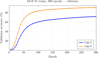
The early curve is the EMA, not the model. With the decay held at \(0.99996\) from step \(0\), the shadow still carries \(0.99996^t\) of the random initialization: \(78\% \) of it at epoch 5, \(29\% \) at 25, \(5\% \) at 60, under \(1\% \) from epoch 100. The trainer scores only the shadow, so the first fifty epochs say nothing about the live weights, which the training loss tracks instead. After that it climbs to the end of the schedule without an overfitting turn, and the scored epochs \(280\)–\(300\) average \(71.48\) with the endpoint at the top of a still-rising tail.
The verified path (PJRT)
The verified trainer is apps/imagenette/MainViTImagenet.lean, built as lake build vit-imagenet-verified:
-- Identical backbone, 1000 classes instead of 10.
def vitImagenetVerified : VerifiedNetSpec where
  name       := "ViT-Tiny (ImageNet-1k)"
  slug       := "vitin"
  data       := .imagenet
  shimScript := "generated_vit_tiny_imagenet_shim.py"
  layers     := [ ... the Imagenette stack, 1000-class head ... ]

-- 300 epochs, because that is the schedule the reference number
-- above was measured on. Batch is 256 PER DEVICE, so four
-- replicas give DeiT's global 1024 exactly.
def vitImagenetConfig : VerifiedConfig where
  epochs    := 300
  batchSize := 256
  vitInit   := true  -- timm/DeiT init, as the reference's default recipe above
The head is the only parameter shape that moves, from \(192 \times 10\) to \(192 \times 1000\), which takes the count from 5,526,346 to 5,717,416. The same three kernel #guards that hold ConvNeXt’s two specs together hold these: equal toSpecs.size, equal toSpecs.pop.pop, and a back! of (#[1000], 2). The driver passes what the render does not bake: the \(10^{-3}\) base rate, the EMA at \(0.99996\) with no ramp, the per-epoch schedule from \(10^{-6}\) and the \(10^{-5}\) floor, all host-side.
The collectives are gated one way here. tests/TestViTDpCheck.lean pins the data-parallel step against its single-device peer by handing both replicas the same rows, where the all-reduce mean is an identity. ViT has no BatchNorm, so that identity is exact rather than approximate. But a gate built on duplicated rows is structurally blind to a shard-offset bug, and the check that closes that hole works by giving the replicas genuinely different data. That one covers the Imagenette vit spec and not vitin. Two gates that sound alike are not one property, and this chapter has one and a half of them rather than ConvNeXt’s two.
The regularizer knobs are render variants, and here they compose. Weight-decay exclusion and stochastic depth are spelled wx and drop, EMA is a variant too, and vitin_emadp256x4wxdropeps0000001smxerfbf16 is the render that carries them on top of AdamW and the four-way all-reduce at \(256\) a replica, at LayerNorm \(\varepsilon = 10^{-6}\) (the digits spell the \(\varepsilon \)), the exact GELU (erf) and no clip: four regions, \([\theta \mid m \mid v \mid \mathrm{ema}]\), 831 operands and 200 all-reduces, with an fp32 evaluation forward at the same \(\varepsilon \) beside it. Mixup, CutMix and repeated augmentation never enter the graph at all, because they are data-side and ride the shim.
The smx in the name is the row maximum. Each of the 36 attention softmaxes subtracts its row’s maximum before the \(\exp \), forward and backward, as JAX’s softmax does: the plain \(\exp (s)/\sum \exp (s)\) overflows f32 once a score passes \(88.72\), and attention scores in this net reach \(90\). The shift is in the AST rather than the printer: a shifted constructor for the forward and one for the backward, denoting \(\mathrm{softmax}(s - \max s)\) row by row, with softmax_sub_const proving the shift away (\(\exp (z_j - c)/\sum _k \exp (z_k - c)\) is \(\exp (z_j)/\sum _k \exp (z_k)\)) and rowSoftmaxShiftFlat_eq, den_softmaxRowBackShiftB_eq lifting that to the rendered nodes. It adds exactly \(72 \times 4\) lines to the train step, 36 forward and 36 backward-recompute softmaxes, with the operand count unchanged, and moves a step’s result by less than the render’s own f32 error (\(2.9\times 10^{-4}\) from an f64 reference, against \(3.0\times 10^{-4}\) without the shift). Theorem 156 is stated on the unshifted chain; each shifted node is proved to denote its unshifted peer, but the tie is not restated on the smx render, so on this pair the step is the render’s through that equality rather than a theorem’s, with the EMA tail outside it as before. It runs with:
lake run vit-default-emabf16-4gpu
Table 9-3 is the run.
|
GPU |
Precision |
Per epoch |
Epochs |
Total |
Val top-1 |
Val top-5 |
|
4\(\times \) 3060 (CUDA) |
bf16 |
12.5 min |
300 |
62.6 hr |
\(\mathbf{71.61\% }\) |
\(\mathbf{90.95\% }\) |
Three hundred epochs at \(751\) seconds each, the evaluation of all \(50{,}000\) images inside, no restart and no thermal rest. Rescored at the live region, the final checkpoint gives \(71.73\% \) / \(91.08\% \).
The two paths, side by side
Table 9-4 is the two paths, row by row.
|
reference (JAX) |
verified path (PJRT) |
|
|
lowering |
JAX \(\to \) XLA |
pretty(provenGraph) \(\to \) XLA |
|
Python in the step |
yes |
none |
|
ms/step |
463 |
573 |
|
per epoch |
9.7 min |
12.5 min |
|
total |
48.3 hr |
62.6 hr |
|
Mixup / CutMix draw |
one per global 1024 |
one per 256-row shard |
|
scored |
every fifth epoch |
every epoch |
|
precision |
bf16 block matmuls |
bf16 block matmuls |
|
patch embed + head |
fp32 |
fp32 |
|
evaluation forward |
fp32 |
fp32 |
|
global batch |
1024 (\(4\times 256\)) |
1024 (\(4\times 256\)) |
|
steps/epoch |
1,251 |
1,251 |
|
peak LR / clip |
\(10^{-3}\) / none |
\(10^{-3}\) / none |
|
schedule |
per epoch, \(10^{-6} \to 10^{-5}\) |
per epoch, \(10^{-6} \to 10^{-5}\) |
|
label smoothing |
\(0.1\) |
\(0.1\) |
|
LayerNorm \(\varepsilon \) / GELU |
\(10^{-6}\) / erf |
\(10^{-6}\) / erf |
|
CLS + position init |
\(\sigma = 0.02\) |
\(\sigma = 0.02\) |
|
EMA (scored) |
0.99996, from step 0 |
0.99996, from step 0 |
|
val top-1 |
\(\mathbf{71.64\% }\) |
\(\mathbf{71.61\% }\) |
|
val top-5 |
\(\mathbf{90.98\% }\) |
\(\mathbf{90.95\% }\) |
|
live weights, top-1 / top-5 |
71.87 / 91.12 |
71.73 / 91.08 |
Above the rule sit the lowering, what it costs, and the two things the runs did not share: where the Mixup and CutMix draws are made — once over the global batch on the reference, once per replica’s \(256\) rows on the verified path, whose four producers each mix their own shard, which is also how timm mixes under DDP — and how often the shadow was scored, which changes no weight.
The pair ties. \(-0.03\) on top-1 and \(-0.03\) on top-5 are a tenth of one run’s \(\pm 0.39\) Wilson half-width at \(n = 50{,}000\): at epoch 300 the two score \(35{,}819\) and \(35{,}806\) images correct, thirteen apart, and the means of the scored epochs \(280\)–\(300\) are \(71.48\) and \(71.44\). The route there is not flat. The verified path leads by up to \(+1.4\) points through epoch 125, the lead decays to under two tenths by epoch 200 and to nothing by \(280\), and the training loss runs within \(\pm 0.02\) of the reference’s in every 25-epoch window and within \(\pm 0.01\) from epoch 126 on. The early lead is the shadow’s: at a constant \(0.99996\) both EMAs carry the random initialization through epoch 60, so the first fifty epochs compare two averages of noise, and the shifted softmax, which changes no function, is not where to look for it. Table 9-5 is the selected epochs and Figure 9-6 every five.
|
epoch |
25 |
50 |
100 |
150 |
200 |
250 |
280 |
300 |
|
reference (JAX) |
11.54 |
41.07 |
60.19 |
65.33 |
68.28 |
70.33 |
71.30 |
71.64 |
|
verified path (PJRT) |
12.62 |
41.89 |
61.17 |
65.80 |
68.44 |
70.49 |
71.25 |
71.61 |
|
\(\Delta \) |
\(+1.08\) |
\(+0.82\) |
\(+0.99\) |
\(+0.47\) |
\(+0.16\) |
\(+0.16\) |
\(-0.05\) |
\(-0.03\) |
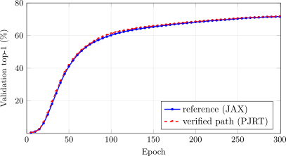
The extra hours are the data feed, not the renderer. The verified step is \(573\) ms against the reference’s \(463\), and the graph itself runs faster than either. The difference is the shim, which augments each image out of process and streams it to the trainer as fp32, about \(600\) MB a step at batch \(1024\), host work the JAX trainer does in-process. The every-epoch evaluation is the rest. The same accounting holds for every verified ImageNet run in this book.
Paired per image, it is still a tie. Both runs score the same \(50{,}000\) images, so the comparison can be made image by image, as §5-5 does. The reference is right on \(2{,}347\) images the verified model misses, and the verified model on \(2{,}327\) the reference misses; McNemar’s exact test gives \(p = 0.78\). The two checkpoints cannot be told apart on this validation set. Matched row for row at DeiT’s own batch, the verified path does not trail its reference.
The live weights are the number DeiT publishes. Scored without the shadow, the reference is \(71.87\) / \(91.12\) and the verified path \(71.73\) / \(91.08\), against DeiT-Ti’s \(72.2\) / \(91.1\), and paired they tie as well (\(p = 0.30\)). On both paths the live weights finish ahead of the shadow. An EMA at \(0.99996\) averages the last twenty epochs of a schedule that is still rising at its end, so it trails the weights it shadows. The tables report the shadow because that is what both trainers score during the run; the live row is the one to read against the paper.
9.6 Side quest: scaling to ViT-S and B
The axis. ViT scales on one axis where ConvNeXt scaled on two. Tiny, Small and Base are the same twelve blocks at a wider model dimension, with the MLP at \(4D\) throughout. Depth never moves. Table 9-6 is the three sizes.
|
model |
shape |
params |
graph, 4 cards \(128\)/dev: fp32 \(\to \) bf16 |
|
ViT-Ti |
\(12\) blocks, \(D{=}192\) / 3 heads |
\(5.7\) M |
\(171.6 \to 96.4\) ms (\(1.78\times \)) |
|
ViT-S |
\(12\) blocks, \(D{=}384\) / 6 heads |
\(22{,}050{,}664\) |
\(464.0 \to 245.5\) ms (\(\mathbf{1.89\times }\)) |
|
ViT-B |
\(12\) blocks, \(D{=}768\) / 12 heads |
\(86{,}567{,}656\) |
\(1295.6 \to 745.3\) ms (\(1.74\times \)) |
Counts #guard against DeiT-S’s \(22.05\) M and DeiT-B’s \(86.57\) M. The times are at four replicas because S and B have no single-device render at all, on the first renders at \(128\) per device. The jobs of Table 9-7 run DeiT’s \(1024\) instead — S as four replicas of \(256\) in one shot, B as two accumulated micro-batches of \(4 \times 128\) — at the \(10^{-3}\) that batch sets, which took one renderer feature, the accumulating optimizer tail, beyond the #eval lines.
A full schedule. Table 9-7 is four cards, \(300\) epochs at the jobs’ own shape — DeiT’s \(1024\), \(1{,}251\) optimizer steps an epoch — with each path’s own trainer timed on real ImageNet (the 2026-10-11 smokes, on the 4060 Ti box).
|
reference (JAX) |
verified path (PJRT) |
|||
|
4 cards, bf16 |
ms/step |
300 epochs |
ms/step |
300 epochs |
|
ViT-S |
\(648\) |
\(72\) h (\(3.0\) d) |
\(650\) |
\(72\) h (\(3.0\) d) |
|
ViT-B |
\(1{,}700\) |
\(180\) h (\(7.5\) d) |
\(1{,}718\) |
\(187\) h (\(7.8\) d) |
The JAX side accumulates two of \(512\), and ViT-B’s verified render two micro-steps of \(4 \times 128\) at \(859\) ms each. These are fed steps, not graph times, and both verified steps are compute-bound, \(9\) and \(5\) ms of them waiting on the shim.
What is queued. Both pairs exist. The verified jobs are vits-default-emabf16-4gpu on vitsin_emadp256x4wxdropeps0000001smxerfbf16, DeiT’s \(1024\) as four replicas of \(256\) in one shot, and vitb-default-emabf16-4gpu on vitbin_emaaccdp2x128x4wxdropeps0000001smxerfbf16, the same \(1024\) as two accumulated micro-batches of \(4 \times 128\), exact under LayerNorm — Tiny’s recipe as §9.5 ran it: vitInit, LayerNorm \(\varepsilon = 10^{-6}\), the \(10^{-5}\) learning-rate floor, EMA at \(0.99996\) constant from step \(0\), no clip, the exact erf GELU, the softmax max-shifted, bf16 under an fp32 patch embedding and head, plus the one row Tiny’s pair ran without: the patch-embedding bias starts at PyTorch’s Conv2d default, \(U(\pm 1/\sqrt{768})\), on both paths — and their references are vits-accum-jax-4gpu and vitb-accum-jax-4gpu, both accumulating \(2\times 512\) to the same \(1024\) (the JAX ViT-S step does not fit the arena in one shot where the verified render does). ViT-S’s render peaks at \(10.75\) GiB of the \(11.68\) GiB default arena; ViT-B’s at \(13.83\) GiB, so its job raises the allocator fraction to \(0.97\) (\(15.11\) GiB).
[TODO: as Tiny’s; neither has run —
vits-accum-jax-4gpu / vits-default-emabf16-4gpu,
vitb-accum-jax-4gpu / vitb-default-emabf16-4gpu.]
9.7 Recap
Attention is \(QK^T\), a softmax over its rows, and a product with \(V\). The softmax Jacobian is a diagonal minus a rank-one correction, the matrix multiply’s backward is two multiplies by transposes, and multi-head attention is those stacked, split and joined. With a vector LayerNorm and the block, the whole ViT-Tiny is proved at depth twelve (Theorem 154) and the network at every depth (Theorem 152): the hand-written input-gradient chain through the patch embedding, twelve blocks, the final LayerNorm and the head equals the network’s Jacobian transpose at every input, assuming only \(\varepsilon {\gt} 0\) at the LayerNorms, and the step is tied (Theorem 156). None of the pieces is new. The height of the composition is. On ImageNet, at DeiT’s own batch, the two paths tie to three hundredths of a point (Table 9-4), and paired per image the tie holds.
Every layer primitive shipped in Part 1’s trainers (MLP, CNN, ResNet, MobileNet, EfficientNet, ConvNeXt, ViT) has a machine-checked backward pass. The same pipeline, a VerifiedNetSpec, a VerifiedConfig and trainAdamSched, trains all of them with at most config-level changes. The MLIR each emits is between 7 KB (MLP) and 1,317 KB (EfficientNet-B0), and the lowerer compiles all of them the same way.
The bestiary in Part 2 then shows that every other architecture you’ve seen in modern deep learning composes from the same small set of primitives plus a handful of architecture-specific bundled layers. That list runs UNet, YOLO, DETR, Mask R-CNN, DCGAN, CycleGAN, Pix2Pix, DDPM, Stable Diffusion, VAE, AlphaGo, AlphaZero, MuZero, Mamba, BERT, GPT, Whisper, CLIP, LLaVA, SAM, SegFormer, DeepLab v3+, Nyström-former, QANet and Evoformer. Three rules (chain, additive fan-in, multiplicative fan-in). Five Jacobian tricks (diagonal, sparse Toeplitz, binary selection, rank-1 correction, outer product).
That’s the whole framework. Part 2’s bestiary takes the same set of primitives and tours how they compose into every well-known modern architecture, a survey of the field expressed in the proven kit, with a small library of bundled idioms for the patterns that recur.