5 ResNet-34

Deeper networks used to stop training

Before 2015, the dominant assumption in image classification was “deeper is better, up to a point.” The “up to a point” part was not metaphorical. If you took a 20-layer CNN that trained to 70% val accuracy and added 12 more convolutional layers, you didn’t get a 32-layer model with 72% accuracy. You got a 32-layer model that, after the same training budget, fit the training set worse than the 20-layer one did. The 32-layer model had strictly more capacity. It still trained worse. Something about deep stacks of convolutions made gradient flow degrade in a way that the optimizer couldn’t navigate around.

He et al. 2015 (arXiv:1512.03385) had the right observation: if the 12 extra layers in the deeper network were initialized to compute the identity, the 32-layer network would have at least the 20-layer’s performance, because it could replicate it exactly. So the question was not “can a deep network represent what a shallow one represents?” It provably could. The question was: why is optimizing 12 free-form layers to recover identity so much harder than just leaving identity there?

5.1 Run it first

Before any of the math, train the thing. Four commands and about fifty minutes of GPU time:

lake exe cache get                            # Mathlib oleans, ~30 s
./scripts/datasets/download_imagenette.sh     # 330 MB dl, 2.4 GB unpacked
lake build resnet34-verified-adam
./.lake/build/bin/resnet34-verified-adam data

On one RTX 4060 Ti (CUDA 12.9), from runs/2026-09-12-r34-ablation-fp32-seeds/full_s2.log: seed 2 of the five that §5.6 averages, run by the ablation driver’s full arm, which is this binary’s render and recipe under LEAN_MLIR_SEED=2. XLA’s startup banner and the resident-parameter notices are removed, the network description line is wrapped, each interval is wrapped onto an indented continuation, and epochs 5 through 75 are elided:

[pjrt_ffi] XLA backend: PJRT 0.114, 1 device(s)
[pjrt_ffi] command buffers: enabled (CUDA default)
[pjrt_ffi] compiled verified_mlir/resnet34_adam_train_step.mlir
             (@resnet34_adam_train_step, 405 outputs, 1 replica) in 6127 ms
[pjrt_ffi] compiled verified_mlir/resnet34_fwd.mlir
             (@resnet34_fwd, 1 outputs, 1 replica) in 596 ms
[pjrt_ffi] compiled verified_mlir/resnet34_fwd_eval.mlir
             (@resnet34_fwd_eval, 1 outputs, 1 replica) in 293 ms
Real ResNet-34 on Imagenette 224² (7×7-s2 stem→3×3-s2 overlapping max pool→
  [3,4,6,3] blocks w/ batch-norm, He et al. option-B 1×1 projection shortcuts,
  no conv biases; 56→28→14→7→GAP→dense)
  via the VERIFIED renderer → XLA/PJRT → GPU
  xla/pjrt verified_mlir/resnet34_adam_train_step.mlir
  xla/pjrt verified_mlir/resnet34_fwd.mlir
  xla/pjrt verified_mlir/resnet34_fwd_eval.mlir
  train 9469, val 3925; bs 32, ResNet-34 adam
    (cosine+warmup 3ep, baseLR 0.001000), He init
  running-stats BN: 36 layers, 17024 stat floats → eval via @resnet34_fwd_eval
Epoch 1/80: loss=1.971035 lr=0.000333
  epoch 1: val_acc = 1239/3925 = 31.566879%  top5 = 2766/3925 = 70.471338%
    [95% CI 30.13–33.04]
Epoch 2/80: loss=1.553382 lr=0.000667
  epoch 2: val_acc = 1471/3925 = 37.477707%  top5 = 3123/3925 = 79.566879%
    [95% CI 35.98–39.00]
Epoch 3/80: loss=1.381944 lr=0.001000
  epoch 3: val_acc = 1880/3925 = 47.898089%  top5 = 3159/3925 = 80.484076%
    [95% CI 46.34–49.46]
Epoch 4/80: loss=1.311593 lr=0.001000
  epoch 4: val_acc = 1851/3925 = 47.159236%  top5 = 3547/3925 = 90.369427%
    [95% CI 45.60–48.72]
Epoch 76/80: loss=0.502131 lr=0.000007
  epoch 76: val_acc = 3536/3925 = 90.089172%  top5 = 3859/3925 = 98.318471%
    [95% CI 89.11–90.99]
Epoch 79/80: loss=0.502245 lr=0.000000
  epoch 79: val_acc = 3535/3925 = 90.063694%  top5 = 3859/3925 = 98.318471%
    [95% CI 89.09–90.96]
Epoch 80/80: loss=0.502085 lr=0.000000
  epoch 80: val_acc = 3535/3925 = 90.063694%  top5 = 3859/3925 = 98.318471%
    [95% CI 89.09–90.96]
done (trained ResNet-34 adam + cosine/warmup via packed threading).

Eighty epochs at about 35 seconds each, 47 minutes in all, and 90.06% top-1 with 98.32% top-5 on Imagenette’s 3,925-image validation split. This is one seed of five; the five land at \(89.99 \pm 0.32\) top-1 (§5.6), and that mean is the number every later chapter compares against.

The residual block: ask for the difference, not the function

Their fix was a one-line architectural change. Instead of asking each block to learn a function \(y = f(x)\), ask it to learn a function \(y = f(x) + x\). The block’s job is no longer to become the new representation. Its job is to learn what to add to the current representation. At initialization, with randomly-small \(f\), each block is approximately the identity, and a stack of 16 such blocks is approximately a stack of 16 identities, which is to say, approximately the input. The network starts out near-identity at every depth and only gradually takes on structure as \(f\) trains. The optimization problem becomes “what residual should each block add” instead of “what function should each block be,” and the former turns out to be dramatically easier.

The change to the architecture is one + sign. The change to the training dynamics is the difference between “18 layers is about as deep as we can go” and “152 layers trains stably, so let us also add another zero on the ImageNet leaderboard.”

Why the proof is a one-liner

From the framework’s perspective, what is a residual block? \(\mathrm{residual}(x) = f(x) + \mathrm{id}(x)\), a sum of two functions sharing the same input. The VJP of an additive fan-in is “send the upstream gradient through both branches and add” (Theorem 11); the VJP of \(\mathrm{id}\) is the identity on the gradient (Theorem 13), and the VJP of \(f\) is whatever the inner block’s machinery gives us. Composition is just \(\mathrm{vjpComp}\). So the residual VJP is the additive fan-in lemma, with \(\mathrm{id}\) plugged into one slot.

That is Theorem 58 below, and its proof is one line. The residual is the one theorem the idea needs, and that theorem is mechanical. The engineering revolution was not in the math. It was in the realization that this operation was the missing piece for training deep networks. The fact that the framework absorbs the new architecture without any new math is the value proposition: once the foundation rules are in place, the next decade of image recognition follows from composing them.

ResNet-34 is sixteen of these blocks

ResNet-34 (the smallest “deep” variant in the original paper) is built from 16 residual blocks arranged in four stages of depths 3, 4, 6, 3, at channel widths 64, 128, 256, 512. Each stage starts with a stride-2 downsample (halving spatial resolution) before its stack of stride-1 blocks. The stages are glued together by a stem (a 7\(\times \)7 conv at stride 2 plus a max-pool, taking 224\(\times \)224\(\times \)3 input to 56\(\times \)56\(\times \)64 features) and a head (global average pool plus a 512-to-10 dense layer). Total: 34 weight-bearing layers, 21.3M parameters.

Two pieces of this template are new and worth naming:

1. The 7\(\times \)7 stride-2 stem. Earlier chapters’ networks operated at full input resolution. ResNet aggressively downsamples at the input so the bulk of compute happens at lower spatial resolution. The stem is one big conv that gets us from 224\(\times \)224 to 56\(\times \)56 in a single step.

2. Global average pool instead of flatten-plus-dense. Chapters 3 and 4 ended in a .flatten followed by a dense layer (\(6272 \to 512\) on MNIST, \(128 \to 512\) on CIFAR) that held most of the network’s parameters. ResNet collapses the final 7\(\times \)7\(\times \)512 feature map to a 512-vector by spatial averaging, then runs a single 512-to-10 dense. No flatten layer. The architectural move alone drops the model from what would have been a \(\sim \)200M-parameter AlexNet-era spec down to 21.3M.

Every chapter after this one is a variation on this template. MobileNetV2 swaps in depthwise-separable blocks. EfficientNet adds squeeze-and-excitation to them. ConvNeXt swaps in its own block. ViT replaces the whole convolutional spine with patches and attention. The stem-stages-head template, and the residual fan-in pattern, persist.

5.2 The theorems

The ladder.

From here every ImageNet chapter proves the same six statements about its network, and this is the first time all six appear. (i) The whole network at batch \(N\) has a VJP: the backward composed from the stages’ backwards is the \(\operatorname {pdiv}\)-contracted Jacobian of the forward. (ii) The hand-written backward chain the renderer emits is that backward. (iii) The emitted training step is the certified step: each of its gradient nodes denotes the certified batch gradient at the chain cotangent of the loss. (iv) Each node is the loss’s derivative in its parameter. (v) The backward is not the zero map, at one fixed weight setting — a seal. (vi) The data-parallel render’s mean over replicas is one device’s step on the global batch. Statements (i), (ii) and (iv) take the smooth-point hypotheses — \(\varepsilon {\gt} 0\) at every BatchNorm, the batch’s activations off every ReLU kink and every pool tie; (iii) and (vi) are identities of the emitted text and take none; (v) is at fixed weights.

5.3 Example: ResNet-34 on Imagenette

ResNet-34 on 224\(\times \)224 Imagenette: 10 classes, real photographs, the transition point from “classroom dataset” to “actual image recognition.”

The architecture

The same vertical column as the previous chapters, now at production scale: a \(7 \times 7\) stride-2 stem and a max-pool drop the \(224 \times 224 \times 3\) input to \(56 \times 56 \times 64\), then four stages of residual blocks (depths \(3, 4, 6, 3\) at widths \(64, 128, 256, 512\)) do the work, and a global average pool replaces the flatten-plus-fat-dense head. The inset shows the one new piece: each residual block adds its input back, \(y = f(x) + x\).

The verified trainer, which is the pattern every later chapter reuses

This is the reference configuration; Chapters 6 through 9 each swap the layers list and change almost nothing else.

import LeanMlir.Verified.NetsCore
import LeanMlir.Verified.Train

-- 1. The network. A VerifiedNetSpec, not a NetSpec: `slug` names the
--    committed render, and `bnChannels` drives BN statistic threading.
def resnet34Verified : VerifiedNetSpec where
  name     := "ResNet-34"
  slug     := "resnet34"
  inC      := 3
  imageH   := 224
  imageW   := 224
  data     := .imagenette
  layers   := [
    .convBnNB 3 64 7 2,          -- 7x7-s2 stem, no conv bias   224->112
    .maxPool 3 2,                -- He et al. 3x3-s2 OVERLAPPING 112->56
    .residualStage  64  64 3 1,  -- stage 1, 3 blocks            @56
    .residualStage  64 128 4 2,  -- stage 2, downsample + 3      56->28
    .residualStage 128 256 6 2,  -- stage 3, downsample + 5      28->14
    .residualStage 256 512 3 2,  -- stage 4, downsample + 2      14->7
    .globalAvgPool,              -- replaces flatten + fat dense
    .dense 512 10 ]
  blurb := "Real ResNet-34 on Imagenette 224² (7×7-s2 stem->3×3-s2 overlapping
            max pool->[3,4,6,3] blocks w/ batch-norm, He et al. option-B 1×1
            projection shortcuts, no conv biases; 56->28->14->7->GAP->dense)
            via the VERIFIED renderer -> %LOWERER% -> GPU"
  bnChannels := #[64, 64,64, ... ]   -- all 36, in forward order

-- 2. The schedule. Everything the optimizer needs beyond the render.
def resnet34AdamConfig : VerifiedConfig where
  epochs    := 80
  batchSize := 32

-- 3. The entry point: AdamW, cosine with a 3-epoch warmup, baseLR 1e-3.
--    Variant, batch and rate are overridable; the defaults are Run it first's.
def runResnet34Adam (argv : List String) : IO Unit := do
  let variant := (← IO.getEnv "LEAN_MLIR_VARIANT").getD "adam"
  let bs      := ((← IO.getEnv "LEAN_MLIR_BATCH").bind (·.toNat?)).getD
                   resnet34AdamConfig.batchSize
  let baseLR := match (← IO.getEnv "LEAN_MLIR_BASE_LR_U").bind (·.toNat?) with
    | some u => u.toFloat * 1e-6     -- micro-units: 100000 is 0.1
    | none   => 0.001
  resnet34Verified.toNet.trainAdamSched
    { resnet34AdamConfig with batchSize := bs }
    (argv.head?.getD "data") baseLR 0.9 0.999 3 variant

The one thing in that listing to carry forward is that the recipe is arguments, not architecture. The learning rate, the momentum pair, the warmup length and the variant string are all passed to the driver; none of them is a property of the network. Swapping AdamW for momentum is a different argument against the same proven gradient, which is what makes §5.6’s ablation a measurement of the recipe rather than of the model — and what Chapter 4 used to put three optimizers on one net.

The schedule. Chapter 4 trained at a constant rate. Annealing the rate to zero on a cosine is worth about five points here (\(-5.00 \pm 2.60\) in §5.6), the largest contribution of any knob in the recipe except augmentation itself, and more than the optimizer, the warmup, the weight decay and the label smoothing combined. It buys that by taking large steps while the loss surface is still coarse and small ones once it is not, which is the reason the warmup exists at the other end and the reason a constant rate has to be a compromise between the two.

This is the first chapter that uses the full production recipe (AdamW + cosine + warmup + weight decay + augmentation + label smoothing). Also the first chapter where .globalAvgPool replaces the flatten-plus-fat-dense head. Global average pooling (GAP) collapses each \(C \times H \times W\) feature map to a length-\(C\) vector by averaging over the spatial dimensions,

so the classifier head sees one summary scalar per channel instead of the full \(C \cdot H \cdot W\) flattened activation.

GAP is not ResNet’s invention. It comes from Network in Network (Lin et al. 2013, arXiv:1312.4400), which proposed it precisely as a replacement for the fully-connected layers at the top of a convolutional net: one feature map per class, averaged, fed straight to the softmax, with no fully-connected parameters to overfit. Inception-v1 (GoogLeNet, Szegedy et al. 2014, arXiv:1409.4842) adopted it a year later — dropping the fully-connected stack for an average pool and a single linear classifier — and reported it worth about \(0.6\% \) top-1 on its own. By 2015 it was standard equipment, which is why ResNet uses it without argument. We’ll see GAP again as the “Squeeze” step inside the squeeze-and-excitation block in Chapter 7, and at the head of every post-2015 vision architecture in the bestiary.

Results

§5.1 has the run: 80 epochs on one RTX 4060 Ti, finishing at 90.06% top-1 and 98.32% top-5 on Imagenette’s 3,925-image validation split, one seed of the five that average \(89.99 \pm 0.32\). That is the going rate for a scratch-trained ResNet-34 at this resolution and data size. From the log:

• Per-step time is about 120 ms at batch 32, 295 steps to the epoch, dominated by the four .residualStage groups where the \(3 \times 3\) convolutions at 64, 128, 256 and 512 channels are. The first stage alone, at 64 channels on the \(56 \times 56\) grid, is \(3 \times 3 \times 64 \times 64\) multiply-accumulates per output location, about \(1.2 \times 10^8\) per convolution, six convolutions in the stage, times the batch, and the backward costs about twice the forward again.

• Final loss plateaus near 0.50, not zero. That’s the label-smoothing floor: with \(\epsilon = 0.1\) and 10 classes, the minimum possible cross-entropy against a smoothed target is \(-0.9 \log 0.9 - 0.1 \log (0.1/9) \approx 0.485\). The 0.50 value at epoch 80 means the model has essentially converged. More epochs would mostly just extend training time without budging the loss.

• BN layers: 36. Every residual block contains two normalized convolutions, and there are 16 blocks across the four stages (3+4+6+3): 32. The projection shortcuts that open stages 2–4 carry one each, and the stem one, for 36 total. Each one proves its own VJP via Theorem 49 and composes with the rest of the network via Theorem 10.

5.4 MLIR: Residual

What is already proven. A residual block is \(\mathrm{residual}(x) = f(x) + x\), an additive fan-in, where \(f\) is the conv \(\to \) BN \(\to \) relu \(\to \) conv \(\to \) BN inner block. As Theorem 58 states, its reverse-mode derivative is the additive-fan-in rule with the identity in one slot: “send the upstream gradient through both branches and add”. residualHasVJPAt proves exactly this at the evaluation point (a one-line proof: the fan-in lemma with the identity’s VJP plugged into one slot), and the inner \(f\)’s VJP is the convolution and BatchNorm backward (Theorems 34, 49). The whole block, and a tower of sixteen of them, composes by the chain rule vjpCompAt (Theorem 10).

The gap and how we close it. The residual fan-in is the structural heart of a deep ResNet. The emitted backward is given a denotation valued in the proofs’ own tensor type, shown equal to residualHasVJPAt’s backward, and the structural move is visible in the emitted text. The forward saves \(\texttt{add} = f(x) + x\) and the block output \(\texttt{relu}(\texttt{add})\). The backward first pushes the incoming cotangent back through that relu (a compare/select at the post-add, giving %dadd), and then, and this is the fan-in, sends %dadd through both branches and adds (the inner block’s forward and \(f\)-backward elided, as they are the conv/BN nodes of Chapters 3–4):

// forward (saved): %out = f(%x)  [conv-BN-relu-conv-BN, Ch. 4-5]
//                  %add = %out + %x
%madd = stablehlo.compare GT, %add, %zc
          : (tensor<1x2x4x4xf32>, tensor<1x2x4x4xf32>)
            -> tensor<1x2x4x4xi1>
%dadd = stablehlo.select %madd, %dOut, %zc
          : tensor<1x2x4x4xi1>, tensor<1x2x4x4xf32>
// %dF = f.backward(%dadd)  [conv/BN/relu input-VJP chain, Ch. 4-5]
%dx = stablehlo.add %dF, %dadd : tensor<1x2x4x4xf32>
return %dx : tensor<1x2x4x4xf32>

Read it against the theorem: %dadd is the cotangent at the fan-in, and it appears twice in the last two lines, once as the input to \(f\)’s backward (%dF, the gradient through the residual function) and once added directly (%dx = %dF + %dadd, the gradient straight down the identity skip). That single stablehlo.add is “send the gradient through both branches and add”: the skip term is the same %dadd the block term started from, which is why the gradient survives all sixteen blocks instead of attenuating away. The inner \(f\) backward that computes %dF, the convolution and BatchNorm input-VJPs, is bridged op by op exactly as in Chapters 3 and 4. Only the fan-in is new here.

Caveats.

• The fan-in add is unconditional, because addition is linear, so that bridge holds at every input.

• The post-add ReLU is a smooth-point bridge (no pre-activation exactly zero), and the two BatchNorms inside \(f\) carry their own \(\epsilon {\gt} 0\) conditions (Theorem 49).

• Representative scale, a two-channel block at \(4\times 4\). The same %dadd fan-in repeats for all sixteen blocks.

5.5 What’s in the production recipe?

Six ingredients first appear here, none of which are layers. They all live in TrainConfig or training code. They don’t touch the network; what each one is worth is measured in §5.6.

Adam (Kingma & Ba, 2014, arXiv:1412.6980). Replaces vanilla SGD. Maintains per-parameter running estimates of the first and second moments of the gradient and uses them for an adaptive per-parameter learning rate. Much faster convergence than SGD on most tasks, much more forgiving of learning-rate choice.

Cosine learning-rate schedule (Loshchilov & Hutter, 2016, arXiv:1608.03983). After warmup, the learning rate decays from its peak to near-zero following \(\mathrm{lr}(t) = \mathrm{lr}_{\max } \cdot \tfrac {1}{2}(1 + \cos (\pi t / T))\). Smoother than step schedules, and consistently produces slightly better final losses in practice. Paired with warmup and progressive resizing (Howard et al., 2018), this was the winning recipe at Stanford’s DAWNBench in 2018. The lineage traces back to Leslie Smith’s cyclical learning rates (Smith 2015, arXiv:1506.01186). Popularized for ImageNet-scale training by He et al. 2018’s “Bag of Tricks” (arXiv:1812.01187).

Warmup (Goyal et al., 2017, arXiv:1706.02677). Linearly ramps the learning rate from zero to its peak over the first few epochs (3 for ResNet-34). Stabilizes early training when gradients are still reorganizing randomly-initialized weights. Becomes essential for larger models and larger batches; Chapter 9’s ViT-Tiny trains with one.

Weight decay. Adds a small L2 shrink to all trainable weights each step: \(w \leftarrow w - \eta \lambda w\), with \(\lambda = 10^{-4}\) here. Regularizer, discourages weights from growing without bound. Loshchilov & Hutter’s “decoupled” variant (AdamW, 2017, arXiv:1711.05101) is what actually ships in modern pipelines, and it’s what TrainConfig.weightDecay implements.

Augmentation. Our pipeline does random crops (\(256 \to 224\)) and random horizontal flips on Imagenette, hflip only on CIFAR, and nothing on MNIST. Lives in the data pipeline, not the network. We will explore data augmentation strategies in upcoming chapters.

Label smoothing (Szegedy et al., 2016, arXiv:1512.00567). Replaces the one-hot target with a smoothed \((\varepsilon / (K-1), \ldots , 1 - \varepsilon , \ldots )\). Stops the network from producing arbitrarily large logits on the correct class, which keeps training stable and improves calibration. Explains the 0.50 loss floor in the Results section above: \(-0.9 \log 0.9 - 0.1 \log (0.1/9) \approx 0.485\).

Every chapter after this one uses the same six ingredients. The NetSpec changes, and the recipe stays.

5.6 Ablation: what each ingredient contributes

So how much does each ingredient actually earn? The full recipe and six leave-one-out variants, ResNet-34 on Imagenette, 80 epochs each. Every variant keeps the recipe intact except for the one component it names, so its difference from the full recipe measures that component’s contribution given everything else is present — not the order-dependent story an additive ladder tells.

Each point is plotted as its difference from the full recipe rather than as an accuracy, so the line at zero is the baseline and distance from it is what the ingredient contributes. Each arm was trained five times from five seeds; the point is the mean difference and the bar its 95% interval, paired by seed, since arms sharing a seed share initialization and data order. An arm whose bar crosses zero is not placed, however suggestive its mean. The full recipe lands at \(89.99 \pm 0.32\) (fp32) and \(89.98 \pm 0.15\) (bf16). Rows are sorted by fp32 effect.

The two panels are the same seven arms in the two precisions, and the reason to draw them side by side is that a real effect should not move. None does: every arm’s fp32 mean falls inside the bf16 interval and every bf16 mean inside the fp32 one. Four arms are resolved in both. Label smoothing is resolved in fp32 (\(-0.69 \pm 0.42\)) but not bf16 (\(-0.50 \pm 0.62\)), where the means agree and only the interval is wider. Weight decay is resolved in neither (\(-0.02 \pm 0.61\), \(+0.14 \pm 0.45\)): ten runs do not place it, and the honest reading is that here it earns nothing measurable.

The cosine bar is the widest in both precisions because the constant-rate arm finishes wherever its noisy trajectory happens to be at epoch 80: fp32 seeds spread \(82.0\)–\(86.8\) (sd \(1.93\)), bf16 \(82.6\)–\(87.9\) (sd \(2.18\)). Its contribution is large and imprecise, and both precisions agreeing on how imprecise says the width belongs to the arm, not to either number format.

What the optimizer row is really measuring. Reading the \(-\)AdamW gap as “what the adaptive optimizer buys” assumes its replacement got a rate that suits it. Heavy-ball at \(\mu = 0.9\) multiplies the effective step by \(1/(1-\mu ) = 10\), so the comparison that isolates momentum is against plain SGD at ten times the rate — \(0.1\), not \(0.01\) — where both take the same size step and differ only in whether a velocity carries it.

At a matched step, plain SGD does not merely keep up with momentum — it finishes slightly ahead, by a paired \(+0.403 \pm 0.162\) with all five seeds agreeing in sign. The two lower bars overlap while that difference is resolved, which is no contradiction: the arms share seeds, so their difference is better determined than either rung’s distance from the baseline. The baseline carries no bar for the same reason — its difference from itself is zero on every seed, and its own spread sits inside the other two bars. The trajectories say the same about shape: the two never separate across the eighty epochs.

Momentum is therefore not doing something a velocity-free step cannot; it is taking a bigger one, slightly less well. The \(-2.27 \pm 0.59\) charged to “removing AdamW” is almost entirely the \(10\times \) momentum supplies for free: hold the effective step fixed and the gap closes to \(-1.86 \pm 0.57\), the remainder running the other way.

That is this ablation’s own limit: every non-adaptive row’s difference is partly a claim about how well its learning rate suits it, and an adaptive optimizer’s insensitivity to that rate hides the dependence. The figure measures the recipe as tuned, not its ingredients in isolation.

Augmentation is the largest single contribution (\(-7.33 \pm 0.49\) fp32, \(-7.11 \pm 0.38\) bf16; three times the next-largest knob). Imagenette has 9,469 training images for a 21.3M-parameter network, so without the random crop and flip the model overfits hard. Most of what the rest of the recipe gets credit for is augmentation.

5.7 ImageNet recipe

The Imagenette runs above all trained on \(\sim \)9.5K images for 80 epochs. This section is the same 21.8M-parameter network on 1.28M images and 1000 classes, trained on the standard 90-epoch schedule. The architecture is unchanged. Only the dataset, the output head width, and the training schedule differ.

This section runs it twice. The reference is the Lean\(\to \)JAX trainer of §C.3.2: JAX traces the generated program and hands XLA the graph. The verified path hands XLA pretty(provenGraph) — the rendered artifact the proofs reason about — through the PJRT C API, with no Python at run time. Same architecture, same recipe, same data loader, same compiler; the only difference is who wrote the StableHLO. Every ImageNet section reports the reference first, the verified path second, and then the two side by side.

The recipe in full: SGD with momentum \(0.9\) at batch 256, cosine LR with a 5-epoch warmup from peak \(0.1\), label smoothing \(0.1\), Inception-style random-resized-crop through TensorFlow’s sampler (\(10\)–\(100\% \) of the image area at a \(\frac{3}{4}\)–\(\frac{4}{3}\) aspect ratio, resized to \(224\times 224\)) plus a horizontal flip, and \(\ell _2\) weight decay \(10^{-4}\). SGD with momentum and the weight decay are the original paper’s; the cosine schedule, the warmup, the label smoothing and the random-resized-crop are the “bag of tricks” polish that became standard after 2018.

The reference (JAX)

The reference trainer is jax/MainResnetImagenet.lean, built as lake build resnet34-imagenet, with .imagenet streamed through tfds. It runs in bf16 — the convolutions cast to bfloat16 against fp32 master weights, the classifier head left in fp32 — which is a throughput choice rather than a fidelity one, and is why its column is the faster of the two below.

Global batch 256 as \(4 \times 64\) replicas; the final checkpoint scored over all \(50{,}000\) validation images through an fp32 forward, as the verified path and timm score, and the run’s own bf16 evaluation lands within \(0.01\) of it.

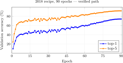
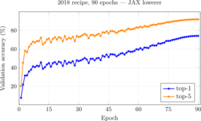
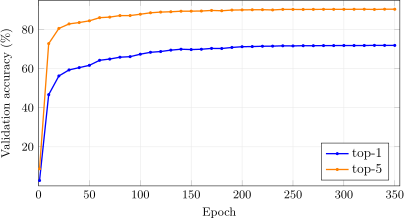
The run, epoch by epoch. The kink near epoch 5 is the end of warmup; the steady late climb is the cosine anneal.

The verified path (PJRT)

The verified trainer is apps/imagenette/MainResnet34Imagenet.lean, built as lake build resnet34-imagenet-verified:

-- 1. Same backbone as the Imagenette net, 1000 classes instead of 10.
def resnet34ImagenetVerified : VerifiedNetSpec where
  name     := "ResNet-34 (ImageNet-1k)"
  slug     := "resnet34in"
  inC      := 3
  imageH   := 224
  imageW   := 224
  data     := .imagenet
  shimScript := "generated_resnet34_imagenet_shim.py"
  layers   := [
    .convBnNB 3 64 7 2,          -- 7x7-s2 stem -> BN -> relu    224->112
    .maxPool 3 2,                -- He et al. 3x3-s2, OVERLAPPING 112->56
    .residualStage  64  64 3 1,  -- stage1: 3 identity            @56
    .residualStage  64 128 4 2,  -- stage2: downsample + 3        56->28
    .residualStage 128 256 6 2,  -- stage3: downsample + 5        28->14
    .residualStage 256 512 3 2,  -- stage4: downsample + 2        14->7
    .globalAvgPool,
    .dense 512 1000 ]
  blurb := "ResNet-34 on full 1000-class ImageNet via the VERIFIED renderer ->
            %LOWERER% -> GPU, with the tfds batch shim supplying the same
            augmentation the Lean->JAX reference trainer uses"
  runningBN := true    -- 36 BatchNorms, read off the layer list

-- The head is the ONLY thing that may differ from the 10-class net.
-- Anything else moving means the spec drifted from its Imagenette twin.
#guard resnet34ImagenetVerified.toSpecs.size == resnet34Verified.toSpecs.size
#guard resnet34ImagenetVerified.toSpecs.pop.pop == resnet34Verified.toSpecs.pop.pop
#guard resnet34ImagenetVerified.toSpecs.back!  == (#[1000], 2)

-- 2. 90 epochs at batch 256.
def resnet34ImagenetConfig : VerifiedConfig where
  epochs    := 90
  batchSize := 256

-- 3. The entry point. Heavy-ball momentum, cosine with a 5-epoch warmup
--    at peak 0.1, weight decay 1e-4, label smoothing 0.1.
-- ⚠ LEAN_MLIR_EPOCHS *sets* the schedule; MAX_EPOCHS only ever CAPS it, and
--    `totalSteps := cfg.epochs * nb / accK` is what the cosine anneals over,
--    so capping at 90 would keep annealing over the default.
def runResnet34Imagenet (argv : List String) : IO Unit := do
  let variant := (← IO.getEnv "LEAN_MLIR_VARIANT").getD "mom256"
  let bs      := ((← IO.getEnv "LEAN_MLIR_BATCH").bind (·.toNat?)).getD
                   resnet34ImagenetConfig.batchSize
  let epochs  := ((← IO.getEnv "LEAN_MLIR_EPOCHS").bind (·.toNat?)).getD
                   resnet34ImagenetConfig.epochs
  let baseLR := match (← IO.getEnv "LEAN_MLIR_BASE_LR_U").bind (·.toNat?) with
    | some u => u.toFloat * 1e-6
    | none   => 0.1
  resnet34ImagenetVerified.toNet.trainAdamSched
    { resnet34ImagenetConfig with batchSize := bs, epochs := epochs }
    (argv.head?.getD "data") baseLR 0.9 0.999 5 variant

Three things in it are worth pulling out, because they are what makes the listing a claim rather than a description.

The slug is the artifact. resnet34in names verified_mlir/resnet34in_<variant>_train_step.mlir — momdp64bf16 for the run below — which is pretty(provenGraph) off the same renderer every earlier chapter used. Scaling to ImageNet needed nothing new in it. nClasses, the batch, the optimizer and the slug are all ordinary parameters, so the ImageNet artifacts are three #evals of machinery that was already proved. What had to be built was the data path, not the compiler.

The #guards pin it to the Imagenette net. The 1000-class spec must be the 10-class one with a different head, and the three guards fail the build if any other parameter shape moves. That is what licenses reading the Imagenette chapter’s theorems as being about this network’s body.

The shimScript is per-net and decides the data. It names this net’s own generated augmentation shim — the same shim the reference consumes, which is what makes the two a matched pair rather than two separate stories.

It runs with:

lake run r34-default-bf16-4gpu

The job config behind that name, scripts/jobs/r34-default-bf16-4gpu.conf, carries the device list, both replica knobs, the variant, the per-replica batch and the feed setting; §3 says what the supervisor behind it does.

Global batch 256 as \(4 \times 64\) replicas, bf16 convolutions under an fp32 classifier head, BatchNorm statistics all-reduced across the four replicas, scored over the same \(50{,}000\) images.

The lowerer underneath is interchangeable. Run from the same initialization, the IREE and XLA lowerings of this artifact scored \(17{,}312\) and \(17{,}313\) correct at epoch 5 — one image apart. The proof-carrying tier reaches this render as a step: Theorems 62 and 68 are stated at either precision, and read over \(\mathbb {R}\) the bf16 text’s gradient nodes are the certified ones. What they do not reach is the rounding: that the hardware rounds where the text says and nowhere else is trusted, as it is at every op of an f32 render.

The two paths, side by side

Both columns are ResNet-34 on the 2018 recipe, 90 epochs, scored over the same \(50{,}000\) validation images under the same protocol. Rows above the first rule differ; rows between the rules are held equal by construction.

The two paths agree to \(0.03\) points on top-1 and \(0.06\) on top-5, and that is well inside what one run can resolve. At \(n = 50{,}000\) the 95% Wilson interval is \(\pm 0.38\) points on either top-1 — \([73.75, 74.52]\) for the reference, \([73.78, 74.55]\) for the verified path — so the gap in the table is a fraction of the interval, and at this scale a gap under about \(0.4\) points is not yet a result in either direction. That is the floor every side-by-side table in this book is read against. Paired on the same images the reading is the same: the two checkpoints disagree on \(5{,}398\) of them, \(2{,}692\) one way and \(2{,}706\) the other, and McNemar’s exact test puts \(p = 0.86\) on the \(14\) images between them.

Both paths normalize over the global \(256\): the reference’s @jit mesh reduces the batch statistics across its shards, and each of the verified render’s 36 BatchNorms all-reduces its mean and variance across the four replicas — the data-parallel step Theorem 68 ties to one device’s step at \(256\).

The curves converge; they do not merely end together. The middle of the schedule is noisy on both paths — at peak learning rate SGD moves top-1 by several points between consecutive epochs, in both directions, six at the worst on either path — so the row is read for its ends. Over the last fifteen epochs the two average within \(0.01\) of each other on top-1 and \(0.02\) on top-5:

One recipe, two paths to XLA, scored over all \(50{,}000\) validation images at every epoch.

A reasonable stopping point

For the fastest path through this book, the route is roughly:

• The intro chapters & Ch 1: framework setup (mandatory context).

• Ch 2–3: MLP and CNN worked examples, the simplest cases of the framework reaching real architectures.

• Skim Ch 4 (BatchNorm). It’s structurally the hardest chapter and the prose says so up front. The math is right (pdiv_bnNormalize’s three-term cancellation is formalized and matches the codegen), but it’s not the place to spend time if you’re not specifically interested in BN. Spend time running as many MNIST and CIFAR demos as possible.

• Read this chapter (Ch 5, ResNet-34). Residual blocks are where the chain rule shows it can carry composition through arbitrarily deep architectures, and the proof reduces to one additive-fan-in lemma you’ve already seen. Run the ResNet-50 RSB-A3 ImageNet training demo (§5.8; about a day on four cards).

• Stop here. Assume Chapters 6–9 (MobileNet, EfficientNet, ConvNeXt, ViT) and the Bestiary (Ch 10) are correct, because they all reuse the same framework with new operators slotting into the same proof tree. Appendix C walks through how that claim is auditable if you ever want to spot-check it.

Reading through Ch 5 is enough to know the framework works. Read the AlphaGo Zero paper (bestiary entry), which combines reinforcement learning with a large residual network of convolutions.

5.8 ResNet-50 on ImageNet: the 2018 recipe and RSB-A3

The basic block ResNet-34 is built from generalizes to the bottleneck block of ResNet-50 — a \(1\times 1\) down, a \(3\times 3\), a \(1\times 1\) back up — at 25.6M parameters against 21.8M. This section moves one lever at a time. First the architecture, with the recipe held fixed: ResNet-50 on the 2018 recipe of §5.7, unchanged, which is worth \(2.7\) points over ResNet-34 on the reference. Then the recipe, with the architecture held fixed: the same network on RSB-A3 (Wightman et al. 2021, “ResNet Strikes Back”), worth about another point. Both recipes run on both paths, so the result is a grid rather than a pair, and the table that closes the section is the 2018 column every later chapter’s recipe is diffed against.

The reference (JAX)

The reference is jax/MainResnet50Imagenet.lean, the bottleneck backbone on the same tfds stream, with the recipe as an argument. The 2018 row is the ResNet-34 recipe with two settings of its own, which A3 keeps: the last BatchNorm \(\gamma \) of each bottleneck starts at zero, and the BatchNorm running statistics decay at \(0.9\) against ResNet-34’s \(0.99\). A3 is LAMB at effective batch 2048 (accumulated as \(4\times 512\)), BCE over Mixup/CutMix targets binarized at timm’s \(0.2\) threshold, RandAugment, and train@160 / eval@224.

Both rows are the final checkpoints scored over all \(50{,}000\) validation images through an fp32 forward, as the verified path and timm score; the trainers’ own bf16 evaluation lands within \(0.04\) of them. A3 normalizes per \(512\)-image micro-batch because it accumulates \(4 \times 512\) to reach \(2048\); the 2018 row is a true global batch of \(256\). That is ghost batch norm (Hoffer, Hubara & Soudry 2017, arXiv:1705.08741): the statistics come from a fixed sub-batch rather than the whole batch, here as a side effect of accumulation rather than a choice, and the A3 render below reproduces it by accumulating the same way. The architecture lever: against ResNet-34’s \(74.14\% \) on the same recipe, the bottleneck is worth \(+2.62\) points. The recipe lever: A3 adds \(+0.99\) on the same network, in less wall clock, because it trains at \(160^2\). It lands \(0.35\) under the paper’s \(78.1\% \) and \(0.30\) under the \(78.05\% \) that timm’s own resnet50.a3_in1k weights score under this protocol, both within one run’s \(\pm 0.36\); what still separates this A3 from timm’s is the marker after the side-by-side table.

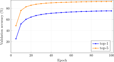
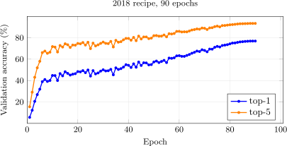
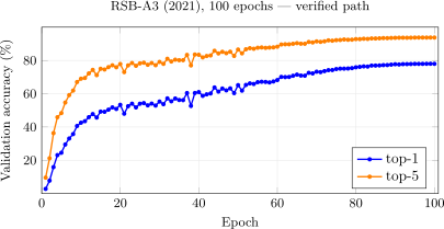
The two recipes on the reference, epoch by epoch. A3 starts far lower — \(1.73\% \) at epoch 1 against \(4.61\% \) — because BCE over mixup targets gives almost no signal until the logits separate; from roughly epoch 35 the two trade the lead, and A3 holds it outright only from epoch 88. At the matched epoch 90 it leads by \(0.45\) (\(77.25\) against \(76.80\)), and its last ten epochs of anneal add the rest. The schedules are different lengths, so at a shared epoch the two cosines are at different points in their decay; the endpoints are what the \(+0.99\) is measured from.

The verified path (PJRT)

The verified trainer is the ResNet-34 one of §5.7 with the bottleneck backbone substituted, and each recipe is its own render: resnet50in_momdp64bf16 for 2018, and for A3 resnet50in160_lambaccdp4x128wxclipbcebf16 — LAMB \(\times \) BCE-with-logits \(\times \) accumulation \(k=4\) at four replicas of \(128\) to the recipe’s \(2048\), train@160 / eval@224. They run with:

lake run r50-2018-bf16-4gpu
lake run r50-a3-wxclip4x128-bf16-4gpu

Scored over the same \(50{,}000\) images. Both renders all-reduce every BatchNorm’s mean and variance across the four replicas (Theorem 69), so the 2018 render normalizes over the global \(256\) and the A3 render over \(4 \times 128 = 512\), the ghost batch the reference’s accumulation gives it.

The A3 render carries the recipe as §5.8 tabulates it, including the three places a bare transcription would miss: BN \(\gamma /\beta \) and biases excluded from weight decay, LAMB’s gradient clip at timm’s default (after the all-reduce and the accumulation, at threshold \(kC\), Proofs.clipFactor_accum), and the no_weight_decay group left out of layer adaptation. The optimizer is tied to the reference at the update as well as the gradient, seven variants to \(\sim \! 10^{-7}\). Both paths run \(625\) steps an epoch and leave \(0.08\% \) of it unused, because \(4 \nmid 2{,}502\). One thing differs from the reference: Mixup’s \(\lambda \) is drawn host-side, once per \(512\)-image micro-batch where the reference draws once per accumulated step, so agreement there is distributional rather than per-step.

The two paths, side by side

Both columns are ResNet-50, each block on its recipe, scored over the same \(50{,}000\) validation images under the same protocol. Rows above the first rule differ; every other row but the results is held equal by construction. The BatchNorm statistic group is the setting that changes between the blocks, on both paths at once: the 2018 recipe normalizes over the global \(256\), and A3 over the \(512\)-image micro-batch its accumulation hands each step — ghost batch norm, on the reference and the verified path alike. [TODO: A3 is timm’s in all but three places, on both paths: Mixup or CutMix drawn per batch at \(p = 0.5\) (ours alternate by step), the schedule stepped once an epoch from \(10^{-4}\) to a floor of \(10^{-6}\) (ours per step from zero), RandAugment’s fill at the image mean (ours grey \(128\)). The \(0.35\) and \(0.19\) to the paper’s \(78.1\) are inside one run’s interval. All three are in code since 2026-10-11, with an fp32 evaluation forward, and not yet run; one rerun of both halves takes them — r50-a3-jax-4gpu / r50-a3-wxclip4x128-bf16-4gpu, \({\sim }13.5 + 24\) h.]

The two paths agree within \(0.33\) points on top-1 on both recipes, and within \(0.06\) on top-5 — inside the 95% Wilson interval, \(\pm 0.37\) at \(77\% \) on \(50{,}000\) images, at one seed per cell. Paired on the same images, the two recipes read differently. On A3 the two checkpoints disagree on \(4{,}014\) images, \(1{,}966\) one way and \(2{,}048\) the other, and McNemar’s exact test puts \(p = 0.20\) on the \(82\) between them: not separable. On 2018 they disagree on \(4{,}622\), \(2{,}228\) against \(2{,}394\), and the \(166\)-image lead is \(p = 0.015\): the verified checkpoint is ahead on this validation set. With one seed per arm that is a statement about two trained models, not about the two paths — the nine percent of images the two disagree on is what two runs of one recipe produce, whichever is ahead — and whether the verified path’s 2018 run is ahead by construction needs seeds per arm. And the recipe delta replicates: A3 beats 2018 by \(+0.99\) on the reference and \(+0.82\) on the verified path. Agreement at a single configuration can be a coincidence of that configuration; a difference that reproduces across two independent implementations is harder to arrange by accident, and it is what a one-row comparison cannot show. One thing the table does not settle: the A3 column trains at \(160\) and evaluates at \(224\) while 2018 does both at \(224\), so the recipe delta confounds resolution with recipe, by A3’s own design.

The 2018 curves travel together; the A3 curves meet. On 2018 the two paths swing both ways through the schedule, as ResNet-34’s do — the verified path minus the reference averages \(+0.22\), \(-0.52\), \(-0.19\), \(+0.07\) and \(+0.24\) over successive twenty-epoch windows, five points apart at the widest. On A3 the verified path runs about a point ahead through the middle of the schedule — \(+1.92\), \(+0.24\), \(+1.16\) and \(+1.05\) by the same windows, ten points at the widest — and the two converge in the anneal, to \(+0.29\) over the last twenty epochs and \(+0.26\) over the last ten. Where A3’s route difference lives is not established; the one difference between its columns that 2018’s do not share is where the Mixup/CutMix draw happens, once per \(512\)-image micro-batch on the verified path against once per accumulated step on the reference, and it is untested. It is why these pairs are read at their endpoints and nowhere else (the rows are the runs’ own per-epoch evaluation through the trainers’ bf16 forward; the headline numbers rescore the final checkpoints through fp32, within \(0.04\) of the last column):

Both recipes on both paths, scored over all \(50{,}000\) validation images at every epoch.

What A3 changes from the 2018 recipe

The 2018-recipe row above is the original paper’s SGD-with-momentum plus the “bag of tricks” polish (cosine schedule, warmup, label smoothing, random-resized-crop). RSB-A3 is the 2021 “ResNet Strikes Back” recipe (Wightman et al.). Both rows are ResNet-50, which is the point: every knob that A3 sets differently is one lever of the three-year jump in how these networks are trained, and holding the architecture fixed is what stops the comparison confounding the recipe with the backbone. The backbone and the entry point are the same for both, and each recipe has its own spec, shim and render. Here is the full diff:

What carries over unchanged: cosine LR decay, the 5-epoch warmup, the base augmentation in the row above, zero-\(\gamma \) initialization, bf16 convolution under an fp32 classifier head, and running-BN evaluation. The through-line of the 2018\(\to \)2021 shift is “regularize harder, train bigger”: heavier augmentation (RandAugment + Mixup + CutMix), a loss that accepts soft targets (BCE), an order-of-magnitude more weight decay applied selectively, and a large-batch optimizer (LAMB) to make the longer, noisier training converge, with FixRes buying back the compute the extra epochs would cost. On the reference every one of these is a one-line TrainConfig change; on the verified path each is a render variant or a shim setting on the same backbone, and the \(160\) train resolution is a spec of its own.

5.9 Side quest: the A2 and A1 recipes

A3 is the cheap tier of “ResNet Strikes Back”. The other two — A2 at 300 epochs and A1 at 600, both at \(224^2\) — render on the verified path as a2 and a1 (the reference’s a2-accum and a1), and neither has been run:

Four artifacts: each tier at four replicas of \(128\), in both precisions — under synchronised BatchNorm the recipe’s ghost batch of \(512\) per micro-step, as for A3. A1 is its own render rather than A2’s with a flag: the weight decay is baked into the artifact, \(0.01\) against A2’s \(0.02\).

A full schedule, four cards, each path’s own trainer timed on real ImageNet at the job’s shape — four replicas of \(128\) accumulated four times to \(2048\), \(625\) optimizer steps an epoch:

A step is one optimizer step, four micro-batches. Totals are training steps alone; evaluation adds a few hours a run.

What the two renders carry, and where they stop short of the paper:

[TODO: as A3’s three, plus timm’s index-level RASampler for the \(3\times \) repeats; neither tier has run — r50-a2-bf16-4gpu / r50-a1-bf16-4gpu, r50-a2accum-jax-4gpu / r50-a1-jax-4gpu.]