10 Bestiary of Architectures

bookmarksdepth=2

Part 1 introduced a small set of NetSpec primitives across chapters 1–9 and proved each one’s backward pass:

• Atomic ops: .dense, .flatten, .conv2d, .maxPool, .convBn, .globalAvgPool, plus the Activation enum (Ch 2–5).

• .residualBlock (Ch 5, ResNet-34).

• .invertedResidual (Ch 6, MobileNet V2).

• .mbConv with optional Squeeze-and-Excitation (Ch 7, EfficientNet-B0).

• .convNextStage + .convNextDownsample (Ch 8, ConvNeXt-T).

• .patchEmbed + .transformerEncoder (Ch 9, ViT-Tiny).

Call this the primary-sequence toolbox — everything a reader has internalized after finishing Part 1. The bestiary is Part 2: a catalogue of famous architectures expressed as pure NetSpec values, no training runs, no VJP commitments, just “here’s what this architecture looks like in \(\sim \)15 lines of Lean.”

What “\(N\) new primitives” means.

Every bestiary entry leads with how many new Layer constructors it asks the reader to absorb on top of the primary-sequence toolbox.

• Zero new primitives means the architecture composes entirely from things you already know — VGG (just \(3\times 3\) conv stacks), AlphaZero (convBn + residualBlock), Highway Networks (two parallel dense paths plus a blend that’s just product rule + additive fan-in from Ch 1). The architecture is conceptually a free read.

• One new primitive means one bundled architectural idiom that wasn’t in Part 1 — .bottleneckBlock for deeper ResNets, .fireModule for SqueezeNet, .mambaBlock for Mamba, etc. The primitive is bundled at the right abstraction level (a whole Mamba block, a stage of Swin attention) so reading it is one chunk, not twenty sub-ops.

• Two or three new primitives are reserved for architectures that genuinely combine multiple novel idioms — DETR (.transformerDecoder + .detrHeads), DenseNet (.denseBlock + .transitionLayer), Stable Diffusion (.unetDown + .unetUp + .transformerDecoder). At most three; if you’d need more, the architecture probably warranted its own chapter.

This count is calibrated to the reader (what’s new vs. what they’ve seen), not to the codebase (where some bestiary primitives were drafted earlier and already sit in Types.lean). Formalizing every sub-op of every modern architecture would be an asymptote we don’t approach.

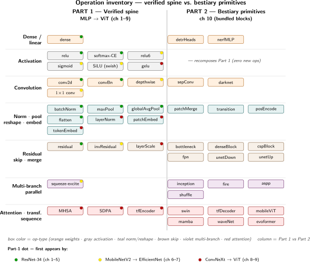
10.1 Bestiary-only Layer primitives

Twenty-five Layer constructors exist only for the bestiary. The two plain ones, .separableConv (Xception, QANet) and .fireModule (SqueezeNet), are described in their entries; the twenty-three bundled ones are defined here. Three of these are codegen-backed, .unetDown and .unetUp, which the segmentation and diffusion demos train through, and .pairTile, the structure demo’s stem; the rest have no emitter, the reference codegen refuses a spec that contains one, and their goal is pedagogical shape and parameter accounting, not training runs.

10.2 Bestiary entries: the chapter nets at work

The entries are grouped by task domain, in two halves. This half is recognition: the chapter nets on pictures, at real-world scale and then on real problems — classification backbones first, where every layer is one Part 1 proved, then detection, inspection, sign language, leaves and tumours, each with a dataset, the field’s own baseline to beat, and beside the demo the architectures that field uses. The second half (§ 10.3) leaves recognition behind, and a last section (§ 10.4) plays games against their exact solutions.

10.2.1 Vision classifiers

Image-classification backbones built out of conv / pool / batch-norm / residual / attention / patch-embed — the exact layer kit VJP’d in Part 1. If a chapter of Part 1 proved it, a bestiary entry below puts it to work.

LeNet (Bestiary/LeNet.lean)

Zero new primitives — just conv2d \(+\) maxPool \(+\) dense. The 1998 original (LeCun et al. 1998, IEEE 1998). Variants: LeNet-5 (61K params, the canonical CNN) and LeNet-300-100 (266K params, pure-MLP baseline). Historical importance; still the ground-truth pattern every later CNN riffs on.

def leNet5 : NetSpec where
  name   := "LeNet-5"
  imageH := 32
  imageW := 32
  layers := [
    .conv2d 1 6 5 .valid .relu,           -- 32×32 → 28×28
    .maxPool 2 2,                         -- 28×28 → 14×14
    .conv2d 6 16 5 .valid .relu,          -- 14×14 → 10×10
    .maxPool 2 2,                         -- 10×10 → 5×5
    .flatten,
    .dense (16 * 5 * 5) 120 .relu,        -- 400 → 120
    .dense 120 84 .relu,
    .dense 84 10 .identity                -- 10-class MNIST output
  ]

AlexNet (Bestiary/AlexNet.lean)

Zero new primitives — five convs, three FCs, pools. The 2012 ImageNet winner that restarted modern deep learning (Krizhevsky et al. 2012, NeurIPS 2012). Variants: AlexNet (62M, paper-exact at 60M; the first FC’s fan-in is pinned to the paper’s \(6 \cdot 6 \cdot 256\), while the spec’s own body ends at \(7 \times 7\)) + tiny CIFAR fixture. \(\sim \)58M of the 62M live in the three FC layers, which is precisely why every post-2015 CNN dropped FC stacks for globalAvgPool + one final dense. LRN is omitted (replaced in the field by BatchNorm in 2015); dropout is training-time only.

Krizhevsky trained on two GTX 580 cards (3 GB each) for \(\sim \)6 days, the two-tower model is a hardware constraint, not a design choice. The winning submission combines convnets with KNN sampling and 10-crop test-time averaging.

def alexNet : NetSpec where
  name   := "AlexNet (Krizhevsky 2012)"
  imageH := 227
  imageW := 227
  layers := [
    .convBn 3 96 11 4 .same,              -- 11×11 stride 4
    .maxPool 2 2,                         -- 3×3 stride 2 in paper
    .conv2d 96 256 5 .same .relu,
    .maxPool 2 2,
    .conv2d 256 384 3 .same .relu,
    .conv2d 384 384 3 .same .relu,
    .conv2d 384 256 3 .same .relu,
    .maxPool 2 2,
    .flatten,
    .dense (6 * 6 * 256) 4096 .relu,      -- ~95% of params live here
    .dense 4096 4096 .relu,
    .dense 4096 1000 .identity
  ]

VGG (Bestiary/VGG.lean)

Zero new primitives — pure stacks of \(3\times 3\) convs + max-pool + a heavy dense head. VGG (Simonyan & Zisserman 2014, arXiv:1409.1556) was the deep-CNN era’s reference architecture for two years between AlexNet and ResNet. Its design philosophy reduced to one rule: “always use \(3\times 3\) kernels and add depth.” Two stacked \(3\times 3\)s cover the receptive field of a \(5\times 5\) with \(\sim \)30% fewer params and an extra nonlinearity in the middle; three stacked \(3\times 3\)s match a \(7\times 7\). The whole architecture is just that trick repeated.

All four paper variants:

All paper-exact. The big numbers come almost entirely from the FC head: the first dense layer alone (\(7\times 7\times 512 \to 4096\)) is \(\sim \)102M of the 138M for VGG-16.

def vgg16 : NetSpec where
  name   := "VGG-16"
  imageH := 224
  imageW := 224
  layers := [
    .conv2d 3 64 3 .same .relu, .conv2d 64 64 3 .same .relu,    .maxPool 2 2,
    .conv2d 64 128 3 .same .relu, .conv2d 128 128 3 .same .relu, .maxPool 2 2,
    .conv2d 128 256 3 .same .relu, .conv2d 256 256 3 .same .relu,
    .conv2d 256 256 3 .same .relu,                              .maxPool 2 2,
    .conv2d 256 512 3 .same .relu, .conv2d 512 512 3 .same .relu,
    .conv2d 512 512 3 .same .relu,                              .maxPool 2 2,
    .conv2d 512 512 3 .same .relu, .conv2d 512 512 3 .same .relu,
    .conv2d 512 512 3 .same .relu,                              .maxPool 2 2,
    .flatten,
    .dense (7 * 7 * 512) 4096 .relu,
    .dense 4096 4096 .relu,
    .dense 4096 1000 .identity
  ]

VGG-16 / VGG-19 still appear in production today as feature extractors (perceptual loss, style transfer) — those FC features turn out to encode useful image structure even after the classification head fell out of favor.

Highway Networks (Bestiary/Highway.lean)

Zero new math — the architecture is built entirely from the product rule and additive fan-in (Chapter 1’s toolkit) applied to two parallel dense / conv paths, and zero new primitives: the two paths are two NetSpecs below and the gate-blend is prose (Srivastava, Greff, Schmidhuber 2015, arXiv:1505.00387). Variants: one highway layer at the paper’s width of 50 units, the same layer at width 100, tiny.

A two-headed network: a main path \(H(x)\) (any transformation, typically dense \(+\) ReLU) and a transform gate \(T(x)\) (its own dense \(+\) sigmoid, output in \([0, 1]\)). The output blends the two:

\(T\) learned per element gives the network a continuous knob between “pass through” (\(T \to 0\)) and “transform fully” (\(T \to 1\)). The gradient through the blend is exactly product rule + additive fan-in (Theorems 12, 11), so no new derivation is needed.

def highway50Main : NetSpec where
  name   := "Highway-50 — main path H(x)"
  imageH := 1
  imageW := 1
  layers := [
    .dense 50 50 .relu                           -- H(x)
  ]

def highway50Gate : NetSpec where
  name   := "Highway-50 — transform gate T(x)"
  imageH := 1
  imageW := 1
  layers := [
    .dense 50 50 .identity                       -- T(x), sigmoid applied at blend
  ]

The pedagogical hook: ResNet (Chapter 5) drops the gate altogether and sums both paths, \(y = H(x) + x\). Highway showed in 2015 that some kind of bypass made very deep networks trainable; ResNet showed six months later that the gate could be a constant and you’d save the parameters. ResNet won by simplifying away \(T\), but the underlying calculus is identical — product + additive fan-in either way.

ResNet (Bestiary/ResNet.lean)

One new primitive (.bottleneckBlock). Chapter 5 walks through the basic-block variant ResNet-34 in detail; this entry catalogs the standard ResNet family (He et al. 2015, arXiv:1512.03385). The basic-block variants (R18, R34) stack two \(3\times 3\) convs per residual unit; the bottleneck variants (R50, R101, R152) use \(1\times 1\) reduce \(\to \) \(3\times 3\) work \(\to \) \(1\times 1\) expand around a residual skip — three convs per block instead of two, but the expensive \(3\times 3\) now runs at \(1/4\) the input channels, so per-block parameter count actually drops.

All three share the same stem (\(7\times 7\) stride-2 conv + \(3\times 3\) stride-2 max pool), the same 4-stage layout (channels \(256 \to 512 \to 1024 \to 2048\)), and the same GAP + single-FC head. They differ only in stage block-counts.

def resnet50Imagenet : NetSpec where
  name := "ResNet-50 (ImageNet)"
  convPadStyle := .symmetric   -- torchvision's 7x7/s2 stem padding, not XLA SAME
  imageH := 224
  imageW := 224
  layers := [
    .convBn 3 64 7 2 .same,
    .maxPool 3 2,
    .bottleneckBlock  64  256 3 1,             -- stage 1: 3 blocks
    .bottleneckBlock 256  512 4 2,             -- stage 2: 4
    .bottleneckBlock 512 1024 6 2,             -- stage 3: 6
    .bottleneckBlock 1024 2048 3 2,            -- stage 4: 3
    .globalAvgPool,
    .dense 2048 1000 .identity
  ]

The residual chain rule (Theorem 58) applies to bottleneck-block ResNets too — the bottleneck just composes three convolutions instead of two inside the residual branch. No new math.

The modern ResNet-50 baseline is timm’s “ResNet Strikes Back” A2 recipe (Wightman et al. 2021, arXiv:2110.00476) — LAMB, BCE loss, repeated augmentation — which trains this exact network to \({\sim }79.8\% \) top-1. The JAX reference trainer (jax/MainResnet50Imagenet.lean) wires that recipe: running the cheaper 100-epoch A3 tier end-to-end through the Lean \(\to \) StableHLO \(\to \) JAX pipeline reaches 77.75% top-1 / 93.65% top-5 on ImageNet-1k, \(0.35\) under the A3 paper’s \(78.1\% \); the verified path’s render of the same recipe scores \(77.91\% \).

WRN (Wide ResNet) (Bestiary/WRN.lean)

Zero new primitives — the residual block of Chapter 5, just widened. Zagoruyko & Komodakis 2016 (arXiv:1605.07146) take the ResNet block and turn the depth knob in (40 layers down from 1000+) and the width knob out (multiply every channel count by \(k\), typically 2–10). Result: WRN-40-4 matches the 1001-layer ResNet on CIFAR-10/100 with fewer parameters and several times faster training, and WRN-28-10 (36.5M in the paper) beats it. Width turned out to be a more efficient axis to scale than depth.

All paper-exact. The N-k naming follows the paper: \(N\) is depth (must be \(6n+4\) for some \(n\) to balance the 3-stage design), \(k\) is the widening factor that multiplies the \(16 \to 32 \to 64\) channel sequence to \(16k \to 32k \to 64k\).

def wrn28_10 : NetSpec where
  name   := "WRN-28-10"
  imageH := 32
  imageW := 32
  layers := [
    .convBn 3 16 3 1 .same,                   -- stem
    .residualBlock 16 160 4 1,                -- stage 1: 4 blocks @ 32×32
    .residualBlock 160 320 4 2,               -- stage 2: 4 blocks @ 16×16
    .residualBlock 320 640 4 2,               -- stage 3: 4 blocks @ 8×8
    .globalAvgPool,
    .dense 640 10 .identity
  ]

The paper also adds dropout between the two convs inside each residual block, which we omit (static-graph scope — no per-step masks). The dropout-free WRN variant is also reported in the paper and lands within \(\sim \)0.3% of the dropout one on CIFAR-10.

SqueezeNet (Bestiary/SqueezeNet.lean)

One new primitive (.fireModule). AlexNet-level accuracy in 1.25M params via the fire module (Iandola et al. 2016, arXiv:1602.07360): squeeze 1\(\times \)1 conv followed by parallel expand 1\(\times \)1 + 3\(\times \)3 convs concatenated. The early efficiency-CNN family alongside MobileNet and ShuffleNet.

Both paper-exact, plus a tiny fixture. SqueezeNet 1.1 is the default for downstream use — same accuracy at \(\sim \)2\(\times \) fewer FLOPs — and is what the first book trained.

def squeezeNet1_1 : NetSpec where
  name   := "SqueezeNet 1.1"
  imageH := 224
  imageW := 224
  layers := [
    .convBn 3 64 3 2 .same,                     -- 3×3 stride-2 stem (vs 1.0's 7×7)
    .maxPool 2 2,
    .fireModule 64  16 64  64,                  -- Fire2  → 128
    .fireModule 128 16 64  64,                  -- Fire3
    .maxPool 2 2,                               -- earlier downsample
    .fireModule 128 32 128 128,                 -- Fire4  → 256
    .fireModule 256 32 128 128,                 -- Fire5
    .maxPool 2 2,
    .fireModule 256 48 192 192,                 -- Fire6  → 384
    .fireModule 384 48 192 192,                 -- Fire7
    .fireModule 384 64 256 256,                 -- Fire8  → 512
    .fireModule 512 64 256 256,                 -- Fire9
    .conv2d 512 1000 1 .same .relu,             -- 1×1 to classes
    .globalAvgPool                              -- GAP emits 1000 logits
  ]

GoogLeNet / Inception v1 (Bestiary/Inception.lean)

One new primitive (§ 142). The parallel-branch architecture that won ImageNet 2014 (Szegedy et al. 2014, arXiv:1409.4842). Three durable contributions, each still standard kit:

• 1\(\times \)1 conv as dimension reducer — placed before the expensive 3\(\times \)3 / 5\(\times \)5 branches, it keeps parallel-branch FLOPs tractable. This is the move every later efficiency-CNN family (MobileNet, EfficientNet, ResNet bottleneck, ShuffleNet) builds on.

• Global average pool replaces the FC head (idea cited from Network-in-Network 2013, popularized here). GoogLeNet’s classifier is one globalAvgPool \(\to \) dense, not VGG’s three-stack of 4096-wide FCs — the same head pattern Chapter 5 onward inherits.

• Auxiliary classifiers branched off the middle of the network at training time, providing intermediate gradient signal. A precursor to deep supervision; the bestiary omits them for spec simplicity.

GoogLeNet ships at 7M parameters — \(\sim \)\(20\times \) smaller than VGG-16 at competitive accuracy on ImageNet 2014.

def googLeNet : NetSpec where
  name   := "GoogLeNet (Inception v1)"
  imageH := 224
  imageW := 224
  layers := [
    -- Stem
    .convBn 3 64 7 2 .same,
    .maxPool 2 2,                               -- 56×56
    .convBn 64 64 1 1 .same,
    .convBn 64 192 3 1 .same,
    .maxPool 2 2,                               -- 28×28
    -- Inception 3a, 3b
    .inceptionModule 192 64 96 128 16 32 32,    -- → 256
    .inceptionModule 256 128 128 192 32 96 64,  -- → 480
    .maxPool 2 2,                               -- 14×14
    -- Inception 4a..4e
    .inceptionModule 480 192 96  208 16 48  64,  -- 512
    .inceptionModule 512 160 112 224 24 64  64,  -- 512
    .inceptionModule 512 128 128 256 24 64  64,  -- 512
    .inceptionModule 512 112 144 288 32 64  64,  -- 528
    .inceptionModule 528 256 160 320 32 128 128, -- 832
    .maxPool 2 2,                                -- 7×7
    -- Inception 5a, 5b
    .inceptionModule 832 256 160 320 32 128 128, -- 832
    .inceptionModule 832 384 192 384 48 128 128, -- 1024
    .globalAvgPool,
    .dense 1024 1000 .identity
  ]

Inception v3 / v4 (Bestiary/Inception.lean)

Zero new primitives — reuses § 142. Inception v3 (Szegedy et al. 2015, arXiv:1512.00567) and v4 (2016, arXiv:1602.07261) are recipe-and-refinement papers more than architecture papers. Three contributions worth pulling out from v3:

• Label smoothing: the cross-entropy target is \(0.9\) on the true class and \(0.1 / (\mathrm{nClasses} - 1)\) elsewhere instead of a hard one-hot. Prevents the softmax from collapsing all probability onto the argmax, which improves calibration and ImageNet accuracy. Now standard in every modern recipe (DeiT, ConvNeXt, our own TrainConfig.labelSmoothing).

• Asymmetric factorizations: a 7\(\times \)1 followed by a 1\(\times \)7 conv replaces a single 7\(\times \)7 with the same receptive field at \(\sim \)\(1/3.5\) the FLOPs. Variant blocks include 1\(\times \)3 + 3\(\times \)1 pairs.

• BN-Aux on the auxiliary classifier branch — the auxiliary classifier of v1 was rebranded as a regularizer rather than a gradient-injection mechanism.

Inception v4 layers more refinement on top: a wider initial stem (stem-A / stem-B / stem-C blocks), three Inception module variants specialized per spatial resolution, and a residual variant (Inception-ResNet) tested in the same paper. Variants here: Inception-v3 (23.8M, paper 23M), Inception-v4 (33M, paper 42M — a bit low because our unified .inceptionModule primitive approximates v3/v4’s richer module catalog).

Xception (Bestiary/Xception.lean)

One new primitive (.separableConv). “Extreme Inception” (Chollet 2017, arXiv:1610.02357): every conv is a depthwise-separable conv. The design choice that made MobileNet possible a year later. Variants: Xception (21.9M, paper-exact at 22M), tiny fixture. Residual skips around each block-of-three-sep-convs are implicit in the linear NetSpec.

def xception : NetSpec where
  name   := "Xception"
  imageH := 299
  imageW := 299
  layers := [
    -- Entry flow
    .convBn 3 32 3 2 .same,
    .convBn 32 64 3 1 .same,
    .separableConv 64 128 1, .separableConv 128 128 1,
    .maxPool 2 2,
    .separableConv 128 256 1, .separableConv 256 256 1,
    .maxPool 2 2,
    .separableConv 256 728 1, .separableConv 728 728 1,
    .maxPool 2 2,
    -- Middle flow: 8× (3 sep-convs + implicit residual), linearized
    .separableConv 728 728 1, .separableConv 728 728 1, .separableConv 728 728 1,
    .separableConv 728 728 1, .separableConv 728 728 1, .separableConv 728 728 1,
    .separableConv 728 728 1, .separableConv 728 728 1, .separableConv 728 728 1,
    .separableConv 728 728 1, .separableConv 728 728 1, .separableConv 728 728 1,
    .separableConv 728 728 1, .separableConv 728 728 1, .separableConv 728 728 1,
    .separableConv 728 728 1, .separableConv 728 728 1, .separableConv 728 728 1,
    .separableConv 728 728 1, .separableConv 728 728 1, .separableConv 728 728 1,
    .separableConv 728 728 1, .separableConv 728 728 1, .separableConv 728 728 1,
    -- Exit flow
    .separableConv 728 728  1,
    .separableConv 728 1024 1,
    .maxPool 2 2,
    .separableConv 1024 1536 1,
    .separableConv 1536 2048 1,
    .globalAvgPool,
    .dense 2048 1000 .identity
  ]

DenseNet (Bestiary/DenseNet.lean)

Two new primitives (.denseBlock, .transitionLayer). DenseNet (Huang et al. 2017, arXiv:1608.06993) takes the ResNet bypass idea to its concatenative extreme: every layer in a “dense block” reads the channel-wise concatenation of all preceding layers’ outputs. Each layer adds only growth_rate new channels (32 in the paper), so the per-layer parameter count stays small while feature reuse compounds.

These specs end in a 10-class (Imagenette) classifier, so they sit below the paper’s 1000-class models by that layer. Plus a tiny fixture for testing.

The dense connectivity pattern doesn’t fit a linear NetSpec at the sub-layer granularity (each sub-layer reads a growing concatenation of its predecessors), so the block is bundled as a shape-only primitive Layer.denseBlock ic growth_rate n_layers alongside Layer.transitionLayer ic oc (BN + 1\(\times \)1 conv + 2\(\times \)2 avg-pool, halves channels and spatial between blocks). Same modeling trick we use for mambaBlock, swinStage, evoformerBlock — the architectural novelty is inside the bundled op.

def denseNet121 : NetSpec where
  name   := "DenseNet-121"
  imageH := 224
  imageW := 224
  layers := [
    .convBn 3 64 7 2 .same,                       -- stem 7×7 stride 2
    .maxPool 3 2,                                  -- 3×3 stride 2 → 56×56
    .denseBlock 64 32 6,                           -- → 256 channels
    .transitionLayer 256 128,                      -- → 128 @ 28×28
    .denseBlock 128 32 12,                         -- → 512 channels
    .transitionLayer 512 256,                      -- → 256 @ 14×14
    .denseBlock 256 32 24,                         -- → 1024 channels
    .transitionLayer 1024 512,                     -- → 512 @ 7×7
    .denseBlock 512 32 16,                         -- → 1024 channels
    .globalAvgPool,
    .dense 1024 10 .identity
  ]

The pedagogical hook: DenseNet sits next to ResNet historically (2017 vs 2015) but architecturally generalizes the bypass primitive — ResNet’s \(y = f(x) + x\) becomes \(y_i = f_i([y_0, \ldots , y_{i-1}])\). The cost: activation memory grows quadratically in block depth from the concatenation. Modern CNN architectures (EfficientNet, ConvNeXt) took the per-layer-parameter-efficiency lesson but dropped the all-pairs concatenation in favor of standard residual paths.

ShuffleNet (Bestiary/ShuffleNet.lean)

One new primitive (§ 145). Grouped 1\(\times \)1 convs + channel shuffle (Zhang et al. 2017, arXiv:1707.01083). Variants: ShuffleNet 0.5\(\times \) / 1.0\(\times \) / 2.0\(\times \) at \(g=3\), plus a tiny fixture.

def shuffleNet1x : NetSpec where
  name   := "ShuffleNet 1.0× (g=3)"
  imageH := 224
  imageW := 224
  layers := [
    .convBn 3 24 3 2 .same,                     -- stem
    .maxPool 2 2,
    .shuffleBlock 24  240 3 4,                  -- stage 2
    .shuffleBlock 240 480 3 8,                  -- stage 3
    .shuffleBlock 480 960 3 4,                  -- stage 4
    .globalAvgPool,
    .dense 960 1000 .identity
  ]

ShuffleNet v2 (Bestiary/ShuffleNetV2.lean)

One new primitive (§ 146). The efficient-CNN paper (Ma et al. 2018, arXiv:1807.11164) that called out FLOPs as a bad latency proxy: measured memory-access cost (MAC) directly and derived four practical guidelines (equal channel widths, avoid grouped convs, avoid fragmentation, avoid element-wise ops). v2’s architecture throws out everything in v1 that violated those rules — no grouped 1\(\times \)1 convs, no skip-add — in favor of channel-split + identity + concat + channel-shuffle. Variants: 0.5\(\times \) (1.37M, paper 1.4M), 1.0\(\times \) (2.29M, paper 2.3M), 1.5\(\times \) (3.52M, paper 3.5M), 2.0\(\times \) (7.41M, paper-exact), tiny fixture. All widths within 2% of paper.

def shuffleV2_1_0 : NetSpec where
  name   := "ShuffleNet v2 1.0×"
  imageH := 224
  imageW := 224
  layers := [
    .convBn 3 24 3 2 .same,                     -- stem
    .maxPool 2 2,
    .shuffleV2Block  24 116 4,                  -- stage 2
    .shuffleV2Block 116 232 8,                  -- stage 3
    .shuffleV2Block 232 464 4,                  -- stage 4
    .convBn 464 1024 1 1 .same,                 -- 1×1 head conv→BN→ReLU (Conv5)
    .globalAvgPool,
    .dense 1024 1000 .identity
  ]

MobileViT (Bestiary/MobileViT.lean)

One new primitive (§ 147); reuses existing invertedResidual for the MV2 stages. Hybrid mobile backbone (Mehta & Rastegari 2022, arXiv:2110.02178): MobileNet V2 body with MobileViT blocks replacing some of the deeper inverted-residual stages. Variants: MobileViT-S (5.6M, paper-exact), XS (2.3M), XXS (1.3M), tiny fixture.

def mobileViTS : NetSpec where
  name   := "MobileViT-S"
  imageH := 256
  imageW := 256
  layers := [
    .convBn 3 16 3 2 .same,                     -- stem
    .invertedResidual 16 32 4 1 1,              -- stage 1: MV2
    .invertedResidual 32 64 4 2 3,              -- stage 2: 3× MV2 + downsample
    -- Stage 3: MV2 downsample + MobileViT (d=144, L=2)
    .invertedResidual 64 96 4 2 1,
    .mobileVitBlock 96 144 4 288 2,
    -- Stage 4: MV2 downsample + MobileViT (d=192, L=4)
    .invertedResidual 96 128 4 2 1,
    .mobileVitBlock 128 192 4 384 4,
    -- Stage 5: MV2 downsample + MobileViT (d=240, L=3)
    .invertedResidual 128 160 4 2 1,
    .mobileVitBlock 160 240 4 480 3,
    .convBn 160 640 1 1 .same,                  -- 1×1 expansion conv→BN→ReLU
    .globalAvgPool,
    .dense 640 1000 .identity
  ]

Swin Transformer (Bestiary/SwinT.lean)

Two new primitives (§ 148, § 149). Variants: Swin-T / -S / -B / tiny. Swin-T lands at 28.6M params against the paper’s 28M (Liu et al. 2021, arXiv:2103.14030) exactly.

def swinT : NetSpec where
  name   := "Swin-T"
  imageH := 224
  imageW := 224
  layers := [
    .patchEmbed 3 96 4 3136,                    -- 56×56 patches, dim 96
    .swinStage 96 3 384 7 2,                    -- stage 1: 2 blocks
    .patchMerging 96 192,                       -- 56×56×96 → 28×28×192
    .swinStage 192 6 768 7 2,                   -- stage 2: 2 blocks
    .patchMerging 192 384,                      -- 28×28×192 → 14×14×384
    .swinStage 384 12 1536 7 6,                 -- stage 3: 6 blocks
    .patchMerging 384 768,                      -- 14×14×384 → 7×7×768
    .swinStage 768 24 3072 7 2,                 -- stage 4: 2 blocks
    .globalAvgPool,
    .dense 768 1000 .identity
  ]

10.2.2 Object detection — demo: R34+FPN on VisDrone

Localize and classify. Detection heads are where the linear NetSpec shape starts to creak: multi-scale FPN outputs need a graph, not a list. The bestiary entries show the single-scale view and defer the multi-head refactor to the limitations discussion.

The working detector.

A ResNet-34 backbone, trained by this stack on ImageNet, feeding an FPN top-down neck into three anchor heads at strides \(8/16/32\); DIoU box loss, focal objectness, focal class CE; \(448\) px input, 30 epochs, photometric and box-aware scale augmentation. VisDrone is the harder half of detection: drone-altitude imagery where a median image holds seventy objects and many are \(2\)–\(5\) px after the resize — the regime where a single coarse grid structurally cannot emit the objects, and what makes the multi-scale head of Definition 152 necessary rather than decorative. Scored against VisDrone’s uncapped validation ground truth — all \(38{,}759\) boxes, not the 56-box-truncated training record, which drops \(34.9\% \) of them and is not the benchmark’s protocol. The catalog entry below keeps the paper-exact YOLOv1 shape for the historical record; this is the trained detector beside it.

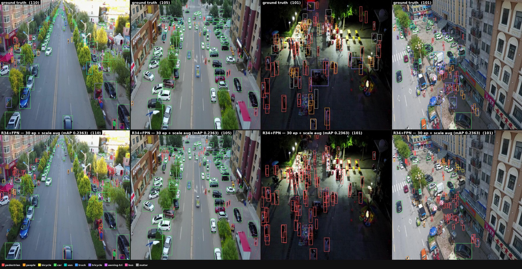
Figure 10.1 is the top row on four validation frames. Augmentation and schedule length are one decision, not two, and the top five rows only mean something together. Quadrupling the schedule with augmentation off costs \(19\% \) — ordinary overfitting on \(6{,}471\) images. Photometric augmentation recovers it, but at that strength 12 epochs still beats 50. Augmentation that changes object scale inverts the ordering again: it makes 30 epochs worth \(44\% \) more than 12. A stronger augmentation needs a longer schedule to absorb, so the optimum epoch count is a property of the augmentation pack — there is no schedule that can be tuned once and carried across packs.

The mean hides where detection fails. Per-class AP runs from car down to bicycle, a spread of \(19\times \), and scale augmentation narrowed it from \(43\times \) by lifting exactly the classes that were worst: awning-tricycle by \(59\% \), bicycle by \(41\% \), tricycle by \(40\% \), against car’s \(7\% \). That the fix was data rather than objective is the substantive point. Reweighting a loss toward rare classes buys their recall at the expense of precision, and average precision charges for the trade; supplying the scales the rare classes are missing raises both at once, which is what the recall and class-agnostic AP columns move together to show. Detection on aerial imagery does not degrade uniformly — it collapses on whatever is simultaneously small and rare, and an averaged mAP is precisely the statistic that hides it.

The stack beats the hand-written PyTorch replica of this same architecture by \(54\% \), and runs at 65 fps on one RTX 4060 Ti — or \(55.9\) fps on a 25 W Jetson Orin Nano under TensorRT, with a uint8 input path and the clocks pinned. The replica, not YOLOv8, is the yardstick: it isolates implementation quality from architecture, which a comparison against a different model would conflate. The two YOLOv8s rows say something more interesting than either alone. At a matched budget it scores \(0.140\) — below this detector, though from random weights rather than an ImageNet-pretrained backbone — while its ordinary-practice \(0.391\) comes from \(8\times \) the epochs, higher resolution, full augmentation and COCO pretraining. The distance to the field is recipe, not architecture, and one item of that recipe closes \(31\% \) of it.

YOLO v1/v3/v5/v8/v11 (Bestiary/YOLO.lean)

v1 (Redmon et al. 2016, arXiv:1506.02640) uses zero new primitives (conv2d + maxPool + flatten + dense; the YOLO-ness lives in the loss and output reshape, not the architecture). v3 adds § 150 for the Darknet-53 body. v5/v8/v11 use § 151 for their CSPDarknet backbones. Variants: YOLOv1 (271M, paper-exact; the first FC’s fan-in is pinned to the paper’s \(7 \cdot 7 \cdot 1024\), while the spec’s own body ends at \(28 \times 28\)), fast, tiny, YOLOv3 (40M backbone), YOLOv5s/m (3M/8M single-scale), YOLOv8n/s (0.7M/2.9M single-scale), YOLOv11n/m (backbone only). Multi-scale FPN detection heads don’t linearize — same skip-connection problem as UNet; all entries show a single-scale view.

def yolo : NetSpec where
  name   := "YOLOv1 (Redmon 2016)"
  imageH := 448
  imageW := 448
  layers := [
    .conv2d 3 64 7 .same .relu,
    .maxPool 2 2,
    .conv2d 64 192 3 .same .relu,
    .maxPool 2 2,
    -- Block 3: 1×1 reduce + 3×3 expand
    .conv2d 192 128 1 .same .relu,
    .conv2d 128 256 3 .same .relu,
    .conv2d 256 256 1 .same .relu,
    .conv2d 256 512 3 .same .relu,
    .maxPool 2 2,
    -- Block 4: four 1×1+3×3 pairs, then 1×1 + 3×3
    .conv2d 512 256 1 .same .relu, .conv2d 256 512 3 .same .relu,
    .conv2d 512 256 1 .same .relu, .conv2d 256 512 3 .same .relu,
    .conv2d 512 256 1 .same .relu, .conv2d 256 512 3 .same .relu,
    .conv2d 512 256 1 .same .relu, .conv2d 256 512 3 .same .relu,
    .conv2d 512 512 1 .same .relu,
    .conv2d 512 1024 3 .same .relu,
    .maxPool 2 2,
    -- Block 5: two 1×1+3×3 pairs + two more 3×3 convs
    .conv2d 1024 512 1 .same .relu, .conv2d 512 1024 3 .same .relu,
    .conv2d 1024 512 1 .same .relu, .conv2d 512 1024 3 .same .relu,
    .conv2d 1024 1024 3 .same .relu,
    .conv2d 1024 1024 3 .same .relu,
    -- Block 6: two 3×3 at 7×7
    .conv2d 1024 1024 3 .same .relu,
    .conv2d 1024 1024 3 .same .relu,
    -- Head: flatten + 2 FC → reshape to (7, 7, 2·5 + 20) = 1470
    .flatten,
    .dense (7 * 7 * 1024) 4096 .relu,
    .dense 4096 yoloHeadSize .identity   -- 7 * 7 * (2 * 5 + 20)
  ]

Mask R-CNN (Bestiary/MaskRCNN.lean)

Two new primitives (.bottleneckBlock + § 152). The canonical two-stage detector + instance segmentation reference (He et al. 2017, arXiv:1703.06870). Five architectural pieces: ResNet-FPN backbone, RPN for anchor-box proposals, ROI-Align for per-proposal feature extraction (an orchestration step, not a layer), a 2-layer FC box head for classification + bbox regression, and a 4-conv + transposed-conv mask head for per-class \(28 \times 28\) masks. Shown as separate NetSpecs per head (SAM-style decomposition). Param totals: backbone+FPN 45.8M, box head 14.3M, mask head 2.6M, RPN 0.6M — \(\sim \)63M in total, matching paper. The FPN cross-scale add is the one thing that demanded a new bundled primitive; everything else reuses existing ResNet / conv / dense primitives. DETR is its end-to-end transformer-era cousin; Mask2Former is the DETR-style instance-segmentation successor.

def maskRCNNBackboneR101 : NetSpec where
  name   := "Mask R-CNN backbone (ResNet-101-FPN)"
  imageH := 800
  imageW := 800
  layers := [
    -- ResNet-101 stem + body (C2..C5)
    .convBn 3 64 7 2 .same,
    .maxPool 3 2,
    .bottleneckBlock 64   256  3  1,            -- C2
    .bottleneckBlock 256  512  4  2,            -- C3
    .bottleneckBlock 512  1024 23 2,            -- C4
    .bottleneckBlock 1024 2048 3  2,            -- C5
    -- FPN: combines C2–C5 into a 4-level feature pyramid at 256 channels
    .fpnModule 256 512 1024 2048 256
  ]

DETR (Bestiary/DETR.lean)

Two new primitives (§ 153, § 154; Carion et al. 2020, arXiv:2005.12872); reuses existing bottleneckBlock (ResNet backbone), patchEmbed (absorbs the DETR 1\(\times \)1 channel reduce), and transformerEncoder. Variants: DETR-R50 (41M, paper-exact), DETR-R101 (60M), tiny.

def detrR50 : NetSpec where
  name   := "DETR-R50"
  imageH := 800
  imageW := 800
  layers := [
    -- ResNet-50 backbone (stem + 4 stages)
    .convBn 3 64 7 2 .same,
    .maxPool 2 2,
    .bottleneckBlock 64 256 3 1,                -- C2
    .bottleneckBlock 256 512 4 2,               -- C3
    .bottleneckBlock 512 1024 6 2,              -- C4
    .bottleneckBlock 1024 2048 3 2,             -- C5
    -- Channel projection (2048→256) + flatten spatial + pos embed
    .patchEmbed 2048 256 1 625,                 -- 25×25 = 625 tokens
    .transformerEncoder 256 8 2048 6,           -- 6 encoder blocks, 8 heads
    .transformerDecoder 256 8 2048 6 100,       -- 6 decoder blocks, 100 queries
    .detrHeads 256 91                           -- class (→92) + box (→4)
  ]

10.2.3 Industrial inspection — demo: the same detector on NEU-DET steel defects

The detector of the previous section, unchanged — backbone, neck, heads, loss, ImageNet bootstrap, scorer — on the dataset the industrial-inspection literature reports on. NEU-DET (Song & Yan 2013; boxes He et al. 2020) is \(1{,}800\) grayscale \(200\times 200\) crops of hot-rolled steel strip, \(300\) per class over six defect types — crazing, inclusion, patches, pitted surface, rolled-in scale, scratches — with Pascal-VOC boxes. It is VisDrone’s opposite regime. A crop holds \(2.3\) defects, half of which span more than half the frame; at the detector’s \(448\) px input, \(98\% \) of the training boxes route to the coarsest pyramid level and none to the finest. This is the dataset on which a single \(14\times 14\) grid should not collapse, and running both heads on both datasets is what shows when multi-scale detection pays.

Three constants change and nothing in the code generation does: the anchor priors are re-fitted to NEU’s boxes (VisDrone’s largest is \(0.18\times 0.15\) of the frame; a steel defect is often half of it), the class weights are off (the data is balanced), and the six classes take ids \(0\)–\(5\) of the ten-slot one-hot, since the \(5+10\) per-anchor width is baked into the fpnDetect emitter and the scorer averages over the classes present. NEU-DET ships no split; the one here is \(1{,}080/360/360\), stratified \(180/60/60\) per class from a fixed seed. Epochs are chosen on the validation \(360\) and the numbers below are the test \(360\) at that epoch, scored by the VisDrone protocol against uncapped ground truth. The single-grid arm is the same ResNet-34 and the same bootstrap under a one-grid YOLOv1 head at \(448/14\), run for the same 30 epochs.

The second table is the result. On steel the single grid matches the multi-scale head, \(0.607\) against \(0.623\); on drones it is six times behind, \(0.039\) against \(0.236\), with recall \(0.18\) against \(0.77\) — same backbone, same bootstrap, same scorer, same lowerer in all four cells. The FPN pays for itself only where objects are small; on NEU-DET it runs three heads for one level’s worth of work, and the head that collapses on VisDrone is not wrong, it is wrong for drones. Recall is not the limit on steel: the FPN finds \(99\% \) of defects and the mean is held down by two classes, crazing at \(0.29\) and rolled-in scale at \(0.41\) against \(0.66\)–\(0.84\) for the other four — the diffuse textures whose “box” is most of the crop, the worst two in every published NEU-DET table and the worst two for both heads here. The ImageNet prefix is worth \(+0.07\) at \(1{,}080\) training images, a gap that has not closed by epoch 30. Photometric augmentation’s \(+0.007\) is one run against one run; no seed spread has been measured on this detector, so it is not a result in either direction.

The distance to the published rows is recipe. Those detectors run at \(640\) px for 300 epochs on a \(1{,}440/180/180\) split; this one runs at \(448\) px for 30 epochs, which on \(1{,}080\) images is \(4{,}050\) steps against VisDrone’s \(24{,}000\), and both arms are still rising at epoch 30. The anchor priors are a second, smaller part of it: three per level fit a level that carries \(98\% \) of the boxes at every aspect from \(64\) px to the full frame at a mean IoU of \(0.52\), and the head has to regress the rest. Both are levers the detector already has; neither was pulled, because the comparison the section makes needs the detector to be the detector.

10.2.4 People watching — demo: Arabic sign-language letters on ArASL

Networks whose input is a person: a face, a gait, a hand. The demo is Chapter 4’s CIFAR net on the dataset the Arabic sign-language literature reports on, run twice on the same images — once under the split every published number uses, once under a split that keeps each hand’s frames together — and the pair of numbers is the result. ArASL (Latif et al. 2019, Data in Brief 23; Mendeley y7pckrw6z2, CC BY 4.0) is \(54{,}049\) grayscale \(64\times 64\) crops of static hand signs for the 32 letters of the Arabic alphabet, \(1{,}293\) to \(2{,}114\) per class, performed by “more than 40 people”. Published classifiers score \(96.6\)–\(97.6\% \) for CNNs trained from scratch (Latif et al. 2020; Alani & Cosma 2021; Abdelghfar et al. 2023) and \(99.3\)–\(99.6\% \) for transfer-learned EfficientNets and ViTs (Al Nabih et al. 2024; arXiv:2410.00681; arXiv:2501.08169), all on random splits. The images are video bursts: sorted by file number within a class, consecutive frames differ by a median \(3.3\) grey levels per pixel where a random pair of the same class differs by \(33\), and cutting where the gap exceeds \(6\) leaves \(14{,}336\) chains of \(3.8\) frames. No signer, session or date is recorded. The two protocols are \(80/10/10\) per class from one seed: random, a stratified permutation, and blocked, each class’s capture order cut at the \(80\% \) and \(90\% \) marks with each cut moved to the nearest chain boundary. An audit then measures what the split did: for every test image, the nearest training image of any class at \(16\times 16\). Under random, \(92.3\% \) of test images have a training image within \(6\) grey levels and \(95.7\% \) of those neighbours carry the test image’s own label; under blocked, \(6.4\% \) and \(28.6\% \). The residual \(6\% \) is the same hand returning a median \(306\) files later, which a release without signer ids cannot separate.

Two numbers change in the network and nothing in the code generation does. CIFAR-CNN8-wide-BN as Chapter 4 spells it — eight convolutions in four conv-conv-pool stages at 16, 16, 32, 32 channels into the \(2\times 512\) head — takes a one-channel stem and a 32-way output; on the native \(64\times 64\) input the four pools end at \(4\times 4\), so the flatten is \(512\) wide and the net is \(0.58\) M parameters. The recipe is the gravitational-wave demo’s, unchanged: the ordinary train step with integer labels, Adam at \(10^{-3}\) with one warm-up epoch and cosine decay, batch 64, 30 epochs, no flip (a mirrored hand is a different sign for some letters), five minutes on one card. The chapter’s linear and MLP rungs run through the same loop as the bracket, and the chapter net at its own \(32\times 32\) input checks that the resolution is not the story. Epochs are chosen on the validation tenth and the numbers below are the test tenth at that epoch, three seeds for the chapter net, with a \(95\% \) Wilson interval on the pooled \(\approx 16{,}200\) trials of \(\pm 0.2\) (random) and \(\pm 0.6\) (blocked).

The two columns are the result. Under the literature’s protocol the chapter net scores \(98.6\% \), above every published from-scratch CNN and a point under the transfer-learned transformers; under the blocked split the same net, recipe and seeds score \(77.9\% \). The audit says where the twenty points went. Nine in ten random-split test images have a training image within six grey levels, and on those the net is at \(99.7\% \); on the \(416\) that do not it is \(85.3\% \); and a nearest-neighbour lookup on \(16\times 16\) thumbnails — no parameters, the training image’s label — scores \(95.7\% \) on the random split and \(28.6\% \) on the blocked one. The published \(96\)–\(99\% \) is mostly the frame, not the hand. The bracket says the same thing from below: the linear classifier loses \(38\) points between the columns and the MLP \(53\), because a pixel-space model can only memorise the hand it saw, and the convolutions lose \(21\), which is the part of the letter they read. The chapter net at its own \(32\times 32\) input loses half a point on the random split and seven more on the blocked one — the difference between hands lives at a resolution the difference between frames does not need. Per class, the blocked column runs from \(16.5\% \) (fa) to \(100\% \) (sheen): the last tenth of some classes’ capture order is a hand no training frame covers, and the classes farthest from their nearest training image are among the worst, but not all the far ones fail — al and seen sit as far from training as fa does and score \(94\% \) and \(100\% \). The rest is which letter the new hand’s shape lands near: fa is called gaaf \(181\) times in three runs and gaaf is called fa once, and taa and thaa, which differ by one raised finger, confuse in both directions.

Two caveats belong beside the number. The blocked split is a proxy for a signer split, not one: the release records no signer, the validation tenth sits next to the training tenths in capture order and is \(37.5\% \) leaked against the test tenth’s \(6.4\% \) (every blocked run shows validation near \(92\% \) and test near \(78\% \), and the epoch is chosen on the leakier of the two), and the \(6\% \) of test hands that return from earlier in the numbering is a floor the protocol cannot remove. And what this classifier is not: it reads one static handshape per frame — fingerspelling, no motion, no grammar, no continuous signing — and the honest number for even that task on new hands is the right-hand column.

10.2.5 Agriculture — demo: lab leaves to field leaves on PlantVillage and PlantDoc

Networks that look at crops. The demo trains a leaf-disease classifier on the dataset the agriculture literature uses most, reproduces its famous number, and then asks the two questions that number does not answer: what does the same net score on a photograph taken in a field, and what was it looking at.

The data. PlantVillage (Hughes & Salathé 2015; Mohanty, Hughes & Salathé 2016; CC BY-SA 3.0) is \(54{,}305\) photographs of single picked leaves laid on a grey background in a laboratory: 38 classes over 14 crops — apple scab, tomato early blight, corn rust, grape black rot, and the healthy leaf of each crop. Published classifiers score \(99\)–\(99.7\% \) on a random split of it. PlantDoc (Singh et al. 2020; CC BY 4.0) is \(2{,}578\) photographs of the same crops and diseases taken where they grow — leaves on the plant, several per frame, soil and sky behind them, phone lighting — in 28 classes that all map onto PlantVillage’s. The net here is Chapter 5’s ResNet-34 from its ImageNet weights with a 38-way head, ten epochs on PlantVillage, forty minutes on one card; PlantDoc is never seen in training except by the last two rows of the table, which learn from it five-fold and are scored only on field images they did not train on. (A near-duplicate audit of PlantVillage finds none, and the maintainers’ own leaf-grouped split gives the same number as a random one; whatever the lab number hides, it is not a repeated frame.)

The first two columns are the result. The net that scores \(99.6\% \) in the laboratory scores \(18\% \) in the field (\(2{,}578\) images, 28 classes, chance \(3.6\% \)). Nothing was wrong with the training; the distribution was. The rest of the section asks the net what it learned, with three instruments that need only the trained weights and the leaf mask PlantVillage ships with every image.

The upper rows are counterfactuals: the same test leaves, edited. The lower rows are the two explainers. The class-activation map is the usual heat map — the class’s weights applied to the last feature map — and the number is how much of its heat falls inside the leaf. The Shapley value treats the image as a game with two players, the leaf and the background, and asks how much of the class score each is responsible for; with two players it is exact from four forward passes (the image, the leaf alone, the background alone, neither), and the two shares add up to the whole score. Both explainers say the same reassuring thing: the evidence is the leaf, \(85\% \) of it. The counterfactuals say otherwise. Put the same leaf on black and the net loses forty points; show it the background with the leaf painted out and it is right one time in four; show it a flat rectangle of the background’s colour and it still beats chance. The background helps in nine images out of ten, a little each time. A map of where the evidence is heaviest does not say what the net cannot do without.

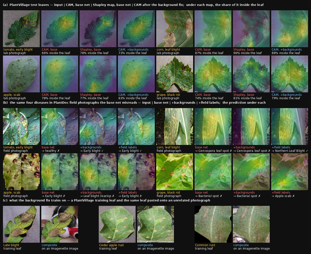
The fixes. Pasting every training leaf onto an unrelated photograph (the composites of panel c) attacks exactly what the table found, and repairs it: the leaves on black go from \(60\% \) to \(96\% \), the background alone falls toward chance, the leaf’s Shapley share rises to \(96\% \). In the field it buys three and a half points, \(17.8 \pm 1.8\) to \(21.5 \pm 1.3\) over three seeds each. Stronger augmentation — colour, rotation, erasing — changes none of the diagnostics and stays inside the seed noise. Field labels are what work: ten per class buy seven points, all two thousand buy twenty-seven, and the two fixes stack only while labels are scarce. The laboratory artefact is real and removable, and removing it is not what gets the net into the field.

What this classifier is not: a diagnosis. It reads one leaf at one moment — no severity, no spread across a field, no symptom before the lesion shows — and the honest number for even that, on a photograph a grower would take, is the right-hand column.

10.2.6 Remote sensing — demo: which wavelengths travel, EuroSAT to the Amazon and the Cerrado

Networks that look down. The demo trains the chapter-4 CNN on satellite chips whose input is not a photograph — thirteen bands of Sentinel-2, ten of them outside what a camera sees — five times, each time allowed a different part of the spectrum, and then asks the trained nets, unchanged, to read land they have never seen. Europe is a target that holds still. The Amazon’s arc of deforestation is a different place, and the Cerrado, read in September and again in March, is a place that moves; the question is which bands can follow it.

The data. EuroSAT (Helber et al. 2019; MIT) is \(27{,}000\) chips of Sentinel-2 imagery over 34 European countries, each \(64\times 64\) pixels at 10 m — a 640 m square — in all 13 bands from 443 to 2190 nm, in ten land-cover classes: annual crop, forest, herbaceous vegetation, highway, industrial, pasture, permanent crop, residential, river, sea or lake. A leaf is bright in the near infrared, where its spongy interior scatters the light that chlorophyll absorbs in the red, and dark in the short-wave infrared, where its water absorbs; the red edge is the step between the two. Colour-infrared film found camouflage on that principle in the 1940s, and the vegetation indices of the 1970s are ratios of exactly these bands. The Brazil chips were cut for this section (data appendix): the same 640 m squares from Sentinel-2 scenes of 2023 over Rondônia in June, and over western Bahia in September and again, the same \(3{,}620\) squares, in March, each labelled by majority vote from MapBiomas, Brazil’s 10 m land-cover map, through the seven classes EuroSAT’s ten collapse into (forest, pasture, herbaceous, annual crop, perennial crop, built, water). The Cerrado’s own class — savanna, woody and herbaceous at once, \(2{,}000\) chips — has no European name and is kept aside. The net is Chapter 4’s CIFAR CNN with the stem’s input channels as the only change: rgb (three bands), rgbn (plus near infrared), ms10 (the ten bands at 10 and 20 m), all (thirteen), and ir (red edge, near and short-wave infrared, and no visible light at all); 80 epochs with flips and rotations, three seeds, five minutes an arm on one card. Nothing in the codegen moves.

The first column is the literature’s question and the second is the demo’s. In Europe the ten invisible bands are worth about a point to a small net trained from scratch, and the bands a camera cannot see are enough on their own (ir, 97.9); the published ordering — RGB 98.6, colour-infrared 98.3, short-wave infrared 97.1 — was the ImageNet pretraining, not the spectrum. In the Amazon the same bands are worth ten. Rondônia is forest and pasture; every arm finds the forest (\(99.8\% \) of it), and RGB loses a quarter of the pasture (\(74\% \) recall) where the ten-band arm keeps \(95\% \). Near infrared alone buys four of the ten points and the red edge and short-wave infrared buy the rest; the arm with no visible light at all reads 91.7.

The Cerrado is the harder question, twice. In September every arm falls to a third, and the confusion is one line of the matrix: a paddock in the dry season is “herbaceous vegetation” to a net that learned pasture from European meadows (RGB puts 666 of 884 there), and the biome’s own class, savanna, is “herbaceous” to all five arms. Merge herbaceous and pasture into one grass class and RGB reads 76; the multispectral arms 65 to 73, because they also send a share of the dry paddocks to “annual crop” — bare, dry ground is a ploughed field in the short-wave infrared. In March the same chips are green, the ten-band arm reads 59 and RGB 38, and savanna becomes “forest” to RGB on \(42\% \) of its chips. The last column is the check the section was built for, and it fails for every arm: the same \(3{,}620\) chips get the same answer in the two seasons between a quarter and two-fifths of the time. The multispectral arms are better in both seasons; they are not stabler. A Cerrado pasture’s red and short-wave reflectance doubles between March and September, and no European chip taught that.

Whose fault. Trained on the Brazil labels themselves, five-fold, the same net reads \(94.2\) with three bands and \(95.8\) with thirteen: the labels are learnable, and the thirteen-band margin over RGB is the same point and a half as in Europe. Fine-tuned from the European weights on 300 Brazilian labels, every arm recovers about 90, the thirteen-band arm a point more; on all of them the European start is worth nothing over scratch. A five-player Shapley value over band groups — visible, red edge, near infrared, short-wave infrared, and the three atmospheric bands at 60 m; a removed group set to its training mean, exact over 32 forward passes per chip — says where the thirteen-band net’s evidence came from: a third of it from visible light on either continent, the short-wave share rising from \(13\% \) at home to \(22\% \) abroad, and the atmospheric bands worth less than nothing in Brazil (\(-3.0\) nats of log-probability in the Amazon). They had learned Europe’s sky, which is why the arm without them travels best.

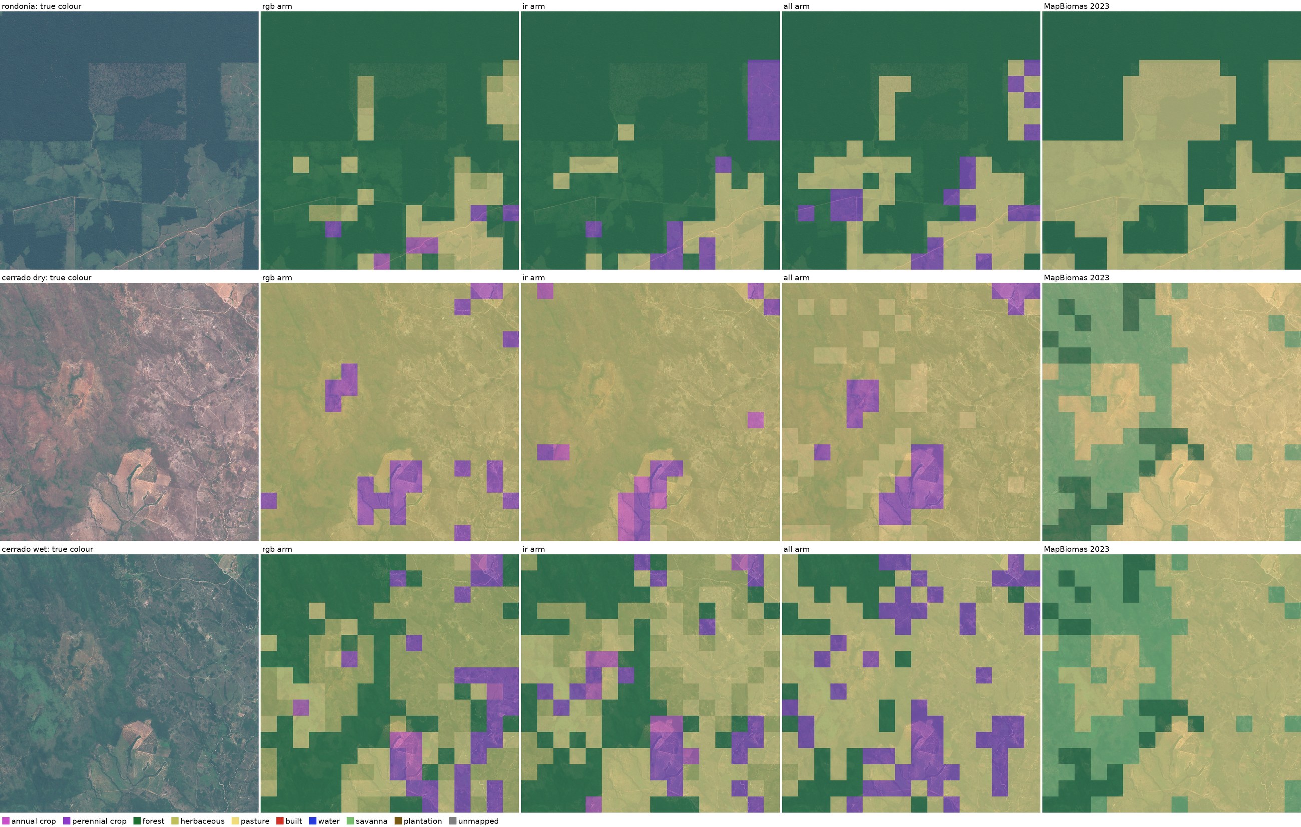
What travelled was the physics: the bands where a leaf’s structure and water are, which read the same over a Bavarian spruce stand and a Rondônia pasture, and carried a net trained on one to the other with no loss worth mentioning. What did not travel was the vocabulary. A class list written for one continent has no word for the other’s biome and a different word for its grass, and the season that turns that grass brown turns every one of these nets around with it. The first is a reason to keep the invisible bands; the second is a reason to label where you look.

What this classifier is not: a map. It says what a 640 m square mostly is — not where the boundary runs, when the forest was cut, or how much of it is gone. The Bahia chips are the first half of the instrument that could say the last two: the same square on two dates, and the difference between them.

10.2.7 Semantic segmentation — demo: UNet on BraTS

Pixel-level labeling. Symmetric encoder/decoder with skip connections is the recurring pattern; UNet is the canonical instance, and the same shape later became the diffusion-model backbone.

A ResNet-34 UNet on BraTS.

The demos/MainUnetBratsR34.lean trainer (unet-brats-r34) is a working encoder–decoder segmentation network at 24.5M params on MSD Task01 brain-tumour MRI: four co-registered modalities (FLAIR / T1w / T1gd / T2w) at \(224 \times 224\) in, four per-pixel classes out (background, edema, non-enhancing/necrotic core, enhancing tumour), 14,415 training slices from 411 patients with the 2,569 validation slices held out by patient. The tumour sub-regions are defined by which modality lights up — edema is bright on FLAIR, enhancing tumour on T1gd — so the input is genuinely multi-modal rather than three correlated views of one scene, and the classes are brutally imbalanced: enhancing tumour is \(\sim \)0.5% of voxels.

Scored on the clinical literature’s regions — Dice over the nested WT (whole tumour), TC (tumour core) and ET (enhancing tumour) — pooled over the 2,569 tumour-bearing validation slices, ten epochs of plain per-pixel cross-entropy gives:

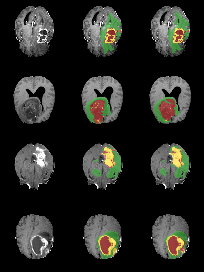
Rendered predictions are Figure 10.6 — T1gd backdrop, ground truth, prediction, on four held-out patients. This matters more than the table for a segmentation demo: a model that has collapsed onto the majority class and one that works report similar pixel accuracy, because 97% of voxels are background. They do not produce similar pictures.

The encoder is the ResNet-34 of Ch 5, reused verbatim as the contracting path rather than a stack of .unetDowns; the decoder is four .unetUp stages, and the skips come off the backbone. The two codegen primitives this rests on — bilinear upsample (forward + VJP) and channel concat — are exposed at the Layer level as .unetDown and .unetUp, which the canonical bestiary UNet below also uses. Three things change relative to the image classifiers of Part 1:

• The label is a tensor, not a scalar. Classifiers emit one logit vector per image (shape \(B \times K\)) and compare it to one ground-truth class. Segmentation networks emit one logit vector per pixel (shape \(B \times K \times H \times W\), with \(H \times W\) matching the input) and compare against a shape-identical ground-truth mask. Cross-entropy is computed per pixel, averaged spatially. This rides the same useSeg flag in TrainConfig that the NLP subsection’s TinyGPT uses for per-token loss, applied across the spatial axes instead of the token axis — no new VJP machinery; the per-pixel softmax-CE backward is the same one Ch 1 derived, fired \(HW\) times in parallel.

• The network has to give spatial resolution back. A classifier downsamples aggressively (input \(224^2\), bottleneck \(7^2\), GAP, \(K\)-way logits) and discards spatial structure on purpose. A segmentation network downsamples and then upsamples, with skip connections from each encoder stage spliced into the matching decoder stage so the output recovers pixel-level detail the bottleneck threw away. That symmetry is exactly what .unetUp’s body bundles — bilinear upsample + channel concat with the saved skip + two convs — and it is the only architectural piece this section’s backbones add to the Part 1 kit.

• Inference is one forward pass; post-processing differs. Segmentation doesn’t autoregress; one network call produces every pixel label simultaneously. What changes is what you do with the logits: argmax per pixel and render as a colored mask. The brats-predict executable is the smallest example of that path — same artifact the trainer produced, plus a small C colormap routine.

What the skips are worth, measured.

The second bullet above is the one claim in this subsection that is cheap to test rather than assert. Running the same backbone, data and schedule with the decoder’s skip connections removed — upsample and convolve, but never concatenate the encoder feature — isolates exactly what they contribute:

Roughly ten points of mIoU, and the largest single gain is on ET (\(+0.12\)), the smallest and thinnest structure — which is what the bullet predicts, since a decoder without skips must reconstruct every boundary from a \(7 \times 7\) bottleneck. It is visible in the renders as well: the thin enhancing rim around the necrotic core is resolved with skips and smeared into the core without them.

Scored per patient.

The tables above pool every pixel of every tumour-bearing slice into one Dice. The literature does something else: one Dice per patient volume, over all of its slices including the tumour-free ones, then the mean over patients — so a small tumour counts as much as a large one, and the slices where there is nothing to paint count against a model that paints anyway. brats-eval (demos/MainBratsEval.lean) computes that from a whole-volume export of the 73 validation patients (preprocess_brats.py –val-full), and first re-derives the pooled number on the same slices, where it agrees with the trainer’s log line to \(0.0004\). Best-by-val checkpoints:

Two things the pooled number hid. The tumour-free slices cost almost nothing: pooled over every slice the Dice is within \(0.003\) of the tumour-slice value, so the slice model does not paint tumour where there is none. And the per-patient mean sits two to seven points below the pooled number with a wide spread (standard deviations of \(0.07\) on WT to \(0.19\) on ET): the medians are at the pooled values, and the means are pulled down by a tail of small-tumour patients — which is what the per-patient protocol exists to expose. The skips are worth more per patient than per pixel, \(+0.17\) on ET against \(+0.12\). These are the numbers to put beside published BraTS work, with the remaining caveat that the 484-case MSD Task01 is not the 1,251-case BraTS 2021 set.

Through-plane context.

A slice model never sees the slice above or below. The last two rows measure what that costs, two ways. unet-brats-r34 ctx=1 is the same net with the two neighbouring slices fed in as eight extra input channels (a 2.5D build from preprocess_brats.py –context 1; the stem is the only tensor that changes, and the records, their order, the seed and the schedule are the 2D run’s): it ties the 2D anchor within \(0.004\) on every metric, pooled and per patient. At 1 mm spacing the neighbours are nearly the centre slice again, so this says adjacent slices add nothing the slice model cannot infer, not that volumetric context is useless. The direct test is a 3D UNet — this section’s UNet with \(3^3\) kernels and \(2^3\) pools, 23.5M parameters — trained in JAX on random \(128^3\) patches for 20,000 steps, a little over five hours on one card (jax/scripts/unet3d_brats.py, the reference a Lean rank-5 port would be tied to). In the table above its means are ahead of the anchor’s by under a point on WT and TC and by two on ET, and most of the ET gain is what a size threshold also buys. So the comparison below applies the usual BraTS post-process to every model — enhancing-tumour predictions under 200 voxels in a volume are relabelled as core — and reads two seeds a side:

The worst tenth is the seven lowest-scoring of the 73 patients, and a false alarm is a slice with no enhancing tumour in the ground truth on which the model paints some, out of 8,060 such slices. Paired over patients the 3D means are ahead by \(0.009\) on WT and TC and \(0.004\) on ET, and the bootstrap interval excludes zero on WT alone. The tail is where the two part. On tumour core the 3D net’s worst tenth is above both 2D seeds’ on both of its own, and it raises a false enhancing-tumour alarm on under half as many slices, a gap twenty times the seed-to-seed spread on either side. On enhancing tumour its worst tenth is ahead on both seeds too, on one of them by less than the two 3D seeds differ from each other. Rank-5 convolution itself runs at 77% of the 2D per-voxel rate through XLA on this card, so the port is affordable; it is not built, and this section’s Lean trainer is the slice model.

Pairing a decoder to a backbone that has no unetDown.

The canonical UNet below pairs skips implicitly — \(i\)-th unetUp from the bottom with \(i\)-th unetDown from the top — which a ResNet encoder cannot satisfy. So unetUp also pairs by shape, with a preceding residual stage or a bare .maxPool’s input; that automatically passes over the bottleneck, which nothing upsamples into. Any ResNet here can therefore be a UNet contracting path. The backward join is .fpnDetect’s C3/C4/C5 tap reused, and routing one network both ways gives bit-identical parameters.

The encoder-decoder-with-skips shape is not specific to segmentation either: it later became the diffusion-model backbone (DDPM, Stable Diffusion, in the diffusion subsection below, §10.3.3), and the same two primitives carry that subsection’s generative pipeline. The layer kit is shared; only the loss and the inference procedure change.

UNet (Bestiary/UNet.lean)

Two new primitives (§ 155, § 156). Skip connections are implicit — the \(i\)-th unetUp from the bottom pairs with the \(i\)-th unetDown from the top. Variants: original (1-channel, 2-class), RGB, small, tiny. Original lands at 31M params matching Ronneberger (Ronneberger et al. 2015, arXiv:1505.04597).

def unet : NetSpec where
  name   := "UNet (original, grayscale → 2-class)"
  imageH := 512
  imageW := 512
  layers := [
    .unetDown 1   64,                           -- encoder stage 1
    .unetDown 64  128,                          -- encoder stage 2
    .unetDown 128 256,                          -- encoder stage 3
    .unetDown 256 512,                          -- encoder stage 4
    .convBn 512 1024 3 1 .same,                 -- bottleneck part 1
    .convBn 1024 1024 3 1 .same,                -- bottleneck part 2
    .unetUp 1024 512,                           -- decoder (skip: encoder 4)
    .unetUp 512 256,                            --         (skip: encoder 3)
    .unetUp 256 128,                            --         (skip: encoder 2)
    .unetUp 128 64,                             --         (skip: encoder 1)
    .conv2d 64 2 1 .same .identity              -- 1×1 conv to 2 classes
  ]

DeepLab v3+ (Bestiary/DeepLabV3Plus.lean)

One new primitive (§ 158). The pre-transformer segmentation workhorse (Chen et al. 2018, arXiv:1802.02611) — still deployed widely in remote sensing, medical imaging, and autonomous-driving perception pipelines. Two ideas: atrous (dilated) convolutions in the backbone’s last stage (param-count-free receptive-field expansion) + an ASPP module for dense multi-scale context at the deepest feature resolution. The “+” in v3+ adds a lightweight decoder that upsamples the ASPP output 4\(\times \) and concatenates a low-level skip from backbone stage 2. Variants: ResNet-101 backbone (59M, paper \(\sim \)63M), MobileNet v2 backbone (5.7M, paper \(\sim \)6M mobile variant), tinyDeepLab fixture. The ASPP skip-to-stage-2 in the decoder doesn’t linearize cleanly; same hack as UNet / WaveNet use. SegFormer (next entry) argues “do ASPP’s multi-scale context via a transformer pyramid”; different mechanism, same goal.

def deeplabv3plusResnet101 : NetSpec where
  name   := "DeepLab v3+ (ResNet-101 backbone)"
  imageH := 513
  imageW := 513
  layers := [
    .convBn 3 64 7 2 .same,                     -- stem
    .maxPool 3 2,
    -- ResNet-101 body; stage 4 uses stride 1 (atrous in real impl)
    .bottleneckBlock 64   256  3  1,
    .bottleneckBlock 256  512  4  2,
    .bottleneckBlock 512  1024 23 2,
    .bottleneckBlock 1024 2048 3  1,
    .asppModule 2048 256,                       -- ASPP: 5 branches + fusion
    -- Decoder (skip from stage 2 doesn't linearize; prose notes it)
    .convBn 256 256 3 1 .same,                  -- 3×3 refine conv→BN→ReLU
    .convBn 256 256 3 1 .same,                  -- 3×3 refine conv→BN→ReLU
    .conv2d 256 21 1 .same .identity            -- Pascal VOC: 21 classes
  ]

SegFormer (Bestiary/SegFormer.lean)

One new primitive (§ 149). Semantic segmentation (Xie et al. 2021, arXiv:2105.15203) via a hierarchical transformer pyramid (MiT encoder: 4 stages of .transformerEncoder glued by .patchMerging) and a lightweight MLP decoder (a handful of .dense calls). The decoder stays trivially small across all B0–B5 encoder sizes — the design argument of the paper is precisely that a good pretrained transformer feature pyramid makes the segmentation head cheap. Variants: MiT-B0 encoder (2.6M, paper 3.7M), B2 (19M, paper 25M), B5 (61M, paper 82M), shared MLP decoder (1M single-scale approx), tiny fixture. Uniform \(\sim \)25% undercount across all encoder sizes because real MiT uses depthwise convs inside the FFN, a strided convolution and norm for spatial-reduction attention, and overlapping patch embeddings at inter-stage transitions; our .transformerEncoder and .patchMerging approximate the shape without those details. Comparison to DeepLab v3+: SegFormer’s decoder is \(\sim \)3M params across all sizes, DeepLab’s ASPP module is \(\sim \)15M and needs per-receptive-field tuning.

def segformerB2 : NetSpec where
  name   := "SegFormer MiT-B2 encoder"
  imageH := 224
  imageW := 224
  layers := [
    -- Stage 1: 224 → 56, 64 channels, 3 blocks
    .patchEmbed 3 64 4 (56 * 56),
    .transformerEncoder 64 1 256 3,
    -- Stage 2: 56 → 28, 128 channels, 4 blocks
    .patchMerging 64 128,
    .transformerEncoder 128 2 512 4,
    -- Stage 3: 28 → 14, 320 channels, 6 blocks
    .patchMerging 128 320,
    .transformerEncoder 320 5 1280 6,
    -- Stage 4: 14 → 7, 512 channels, 3 blocks
    .patchMerging 320 512,
    .transformerEncoder 512 8 2048 3
  ]

SAM (Bestiary/SAM.lean)

One new primitive (§ 153). Promptable segmentation (Kirillov et al. 2023, arXiv:2304.02643): a ViT image encoder runs once per image, a tiny prompt encoder tokenizes clicks / boxes / masks, a lightweight transformer mask decoder cross-attends between image tokens, prompt tokens, and a handful of learned output queries. Image encoder is .patchEmbed + .transformerEncoder (the ViT kit); mask decoder is a small .transformerDecoder (from DETR, 4 queries, 2 blocks). Variants: SAM ViT-B encoder (88M, paper total 91M), ViT-L (307M, paper 308M), ViT-H (635M, paper 636M), shared 3.3M mask decoder, tinySAM fixture. The image encoder accounts for \(\sim \)99% of each variant’s parameter budget, which is why EfficientSAM (Xiong et al. 2023) focused its distillation there.

def samEncoderH : NetSpec where
  name   := "SAM ViT-H image encoder"
  imageH := 1024
  imageW := 1024
  layers := [
    -- 16×16 patches on 1024×1024 → 64×64 = 4096 tokens
    .patchEmbed 3 1280 16 SAM_PATCHES,
    .transformerEncoder 1280 16 5120 32          -- 32 blocks, dim 1280
  ]

10.3 Bestiary entries: beyond recognition

The training signal stops being a label. It is the next token, the noise added to an image, a density, a chirp buried in detector noise, an energy, the distance between two residues of a protein — and where the field has an exact answer, quadrature, the matched filter’s closed form, a solved spin chain, or a blind competition’s table, the demo is scored against it rather than against a held-out set. The networks are the same kit; what changes is the outer loop, and the catalogue beside each demo is that domain’s architectures. The games, whose signal is a reward and whose answers are theorems about the rules, are § 10.4.

10.3.1 Natural language processing — demo: TinyGPT on Shakespeare

The architectures here all consume a sequence of token IDs and emit either a sequence of next-token logits (decoder-only: GPT) or a single classification head (encoder-only: BERT). At the layer level they reduce to one of three shapes: a stack of .transformerEncoder (with or without a causal mask), a state-space stack (.mambaBlock), or a conv/attention hybrid (.separableConv plus .transformerEncoder, QANet). What’s different from the vision side of the bestiary isn’t the layer kit — the kit is the same set of primitives Ch 9 introduced — it’s everything around the layers: the data pipeline, the loss, and the inference loop.

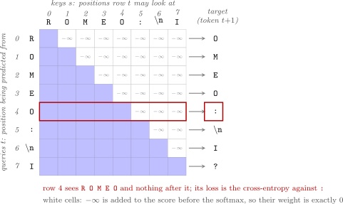
TinyGPT, in passing.

The demos/MainTinyGptShakespeare.lean trainer in this repo is a working char-level transformer at 212K params (\(T{=}64\), \(D{=}64\), 4 layers, 2 heads). Ten thousand Adam steps take three minutes on one RTX 4060 Ti through XLA, compile included, and land at 2.28 bits/char on tinyshakespeare’s held-out split — against 3.56 for a bigram table and 6.02 for guessing uniformly over the 65 characters. Sampling after that produces recognizable Shakespeare cadence, real character names (NORTHUMBERLAND, QUEEN MARGARET, MERCUTIO, BRUTUS) and multi-line dialog. Three things change relative to the image trainers shown throughout Part 1, and they capture what NLP training is:

• Input is a vocabulary index, not a pixel. The first layer of every NLP spec is .tokenPositionEmbed (one-hot \(\to \) learnable token embedding \(+\) learnable position embedding). Image stacks open with .conv2d or .patchEmbed acting on \(H \times W \times 3\) floats; the NLP stack starts with vocabulary IDs flowing through a lookup table. Replace patches with tokens and the rest of a ViT is shape-identical to a GPT.

• Loss is per-token, averaged over the sequence. Image classifiers compute one cross-entropy at the end of the network: pool to a vector, dense to logits, compare to one ground-truth class. Language models compute cross-entropy at every position — each of the \(T\) tokens predicts the next one, and the per-token losses are averaged. Our trainer reuses the same cross-entropy path through a flag (useSeg in TrainConfig) that switches the loss from “one vector versus one class” to “\(T\) vectors versus \(T\) classes.” No new VJP machinery; the per-token softmax-CE backward is the same one Ch 1 derived, applied \(T\) times in parallel.

• Inference is autoregressive. The training loop is a single forward pass per batch, just like image classification, but inference is a \(T\)-step loop: the network predicts token \(t{+}1\) from tokens \([0..t]\), the sampled token is appended to the context, and the network runs again for \(t{+}2\). Our tinygpt-shakespeare sample executable implements exactly this loop — \(\sim \)30 lines of plain Lean, no proof machinery, running the same spec’s forward graph at batch one through XLA on the parameters the trainer saved. The architectural cost is the causal mask (Figure 10.7): during training, attention at position \(t\) must not see positions \(t{+}1\) onward, or the model would trivially predict the answer it can see. We expose this via the causalMask flag on .transformerEncoder; the rest of the kit is shared with ViT.

That’s the entire delta. Same Adam optimizer, same VJP machinery, same StableHLO-through-XLA pipeline. The bestiary entries below all reduce to either “GPT shape” (decoder-only, causal mask, autoregressive sampling) or “BERT shape” (encoder-only, bidirectional attention, classification head); the architectural differences between them are smaller than the chapter-to-chapter deltas in Part 1.

Mamba (Bestiary/Mamba.lean)

One new primitive (§ 159). Variants: Mamba-130M / 370M / 790M / tiny, matching Gu & Dao’s (2023, arXiv:2312.00752) param counts within \(\sim \)5%.

def mamba130M : NetSpec where
  name   := "Mamba-130M"
  imageH := 2048                                  -- context length (L tokens)
  imageW := 1
  layers := [
    -- dim=768, state=16, expand=2, 24 blocks
    .mambaBlock 768 16 2 24,
    .dense 768 50280 .identity                    -- LM head (GPT-NeoX vocab)
  ]

BERT / RoBERTa (Bestiary/BERT.lean)

Zero new primitives — uses .transformerEncoder, same kit as ViT / DETR, plus .dense vocab\(\to \)dim standing in for the token-embedding table (faithful param count, shape semantics cheat since a linear NetSpec can’t express the \(L \to L \times D\) lookup). Variants: BERT-base (109M, paper 110M), BERT-large (335M, paper 340M), RoBERTa-base (124M, paper 125M), RoBERTa-large (355M, paper-exact), tinyBERT fixture. The architectural lesson is that RoBERTa (Liu et al. 2019, arXiv:1907.11692) = BERT (Devlin et al. 2018, arXiv:1810.04805); all RoBERTa gains came from training procedure (dynamic masking, more data, bigger batches, dropped NSP) — none of which lives in the NetSpec.

def bertBase : NetSpec where
  name   := "BERT-base"
  imageH := 512                                   -- max context length
  imageW := 1
  layers := [
    -- Token-embedding lookup approximated as dense (vocab → D)
    .dense 30522 768 .identity,
    -- 12 encoder blocks, post-norm, GELU, mlpDim = 4·D
    .transformerEncoder 768 12 3072 12,
    -- [CLS] pooler (tanh applied downstream)
    .dense 768 768 .identity
  ]

GPT-1 / GPT-2 (Bestiary/GPT.lean)

Zero new primitives. GPT-1 (Radford et al. 2018, OpenAI TR) and GPT-2 (Radford et al. 2019, OpenAI TR) are decoder-only counterparts of BERT. Same .transformerEncoder, now read as a stack of decoder blocks with a causal attention mask (a training-time detail, not a parameter). No pooler; GPT-2 uses pre-norm instead of BERT’s post-norm (zero-parameter swap). Weight tying: the LM head reuses the token-embedding matrix, so our .dense vocab\(\to \)D stand-in already pays for both input and output sides. Variants: GPT-1 (116M, paper 117M), GPT-2 small (123M, paper 124M), medium (353M), large (772M, paper 774M), XL (1.56B, paper 1.5B), tinyGPT fixture. Reference implementation: Karpathy’s nanoGPT (\(\sim \)300 lines of PyTorch) targets GPT-2 small and is the canonical mental model.

def gpt2Small : NetSpec where
  name   := "GPT-2 small"                         -- the nanoGPT target
  imageH := 1024                                  -- context length
  imageW := 1
  layers := [
    -- Tied token embedding (also serves as LM head projection)
    .dense 50257 768 .identity,
    -- 12 decoder blocks, pre-norm (mask is attention-time, not a param)
    .transformerEncoder 768 12 3072 12
  ]

QANet (Bestiary/QANet.lean)

One new primitive (.separableConv). The 2018 reading-comprehension architecture that killed the BiLSTM for SQuAD-style tasks (Yu et al. 2018, arXiv:1804.09541). Core contribution: an encoder block combining 4 depthwise- separable convs (local context) with a self-attention + FFN transformer block (global context) — the “conv + attention hybrid” shape MobileViT and ConvNeXt rediscovered in 2022. Expressed with primitives we already have: 4 .separableConv 128 128 1 calls + 1 .transformerEncoder 128 8 512 1 per block. Per-block count: \(\sim \)270K for the embedding-encoder block; the model-encoder blocks carry two separable convs rather than four, and the paper’s seven-block stack lands at \(\sim \)1.6M, repeated 3 times in the full architecture. The BiDAF- style context-query attention and character/word embedding tables are omitted from the spec; described in prose. QANet’s headline number was 3–4\(\times \) training speedup over BiLSTM-based competitors, a clean example of hardware (parallelization of convs vs. sequential RNN roll-outs) forcing an architectural choice. BERT landing 7 months later ended the SQuAD-as-benchmark era, but QANet’s hybrid shape lived on — showed up repeatedly in vision 4 years later.

def qanetEncoderBlock : NetSpec where
  name   := "QANet encoder block (4× sep-conv + self-attn + FFN)"
  imageH := 400                                   -- representative context length
  imageW := 1
  layers := [
    -- 4 depthwise-separable convs (local context, kernel 7 in paper)
    .separableConv 128 128 1,
    .separableConv 128 128 1,
    .separableConv 128 128 1,
    .separableConv 128 128 1,
    -- Self-attention + FFN + 2 LayerNorms (global context)
    .transformerEncoder 128 8 512 1
  ]

Nyströmformer (Bestiary/Nystromformer.lean)

Zero new primitives. An efficient-attention transformer (Xiong et al. 2021, arXiv:2102.03902) that replaces the \(O(n^2)\) softmax attention with an \(O(n)\) Nyström-approximation computed via \(m\) landmark tokens, \(m \ll n\). Crucially, this is a compute change, not a parameter change: the \(W_Q / W_K / W_V / W_O\) projections and the FFN are identical to a standard transformer. Our .transformerEncoder spec is therefore identical to BERT’s at each scale — base lands at 108M (vs BERT-base 109M), large at 333M (vs BERT-large 335M). The entry’s pedagogical value is prose-level: most of the 2020–2022 efficient-attention literature (Linformer, Performer, Longformer, BigBird, Reformer, FlashAttention) is parameter-identical to vanilla attention, and the bestiary can’t differentiate them at the layer level. Nyströmformer is worth highlighting because the specific trick — a 1930 result from numerical linear algebra, routed through kernel-method literature in the early 2000s, finally surfacing in transformers — is a genuinely long arc for one math idea.

def nystromformerBase : NetSpec where
  name   := "Nyströmformer base (BERT-base-shaped, O(n) attention)"
  imageH := 4096                                  -- long context
  imageW := 1
  layers := [
    -- Architecturally identical to BERT-base; Nyström approximation
    -- lives inside the attention kernel, not the NetSpec.
    .dense 30522 768 .identity,
    .transformerEncoder 768 12 3072 12
  ]

10.3.2 Image generation

Networks whose output is a novel image. Two families covered here: variational autoencoders and GANs. Backbones overlap heavily with segmentation (UNet again). Diffusion models, also generative, are the subsection after this one.

VAE (Bestiary/VAE.lean)

One new primitive (§ 156). The classical variational autoencoder (Kingma & Welling 2013, arXiv:1312.6114): encoder outputs \((\mu , \log \sigma ^2)\) (represented as a single tensor with doubled final width), the reparameterization trick \(z = \mu + \sigma \odot \epsilon \) samples \(z\) in training code, the decoder reconstructs. KL divergence between the learned latent distribution and a standard normal is the regularizer. Variants: MNIST MLP VAE (20-dim latent, textbook example), CIFAR conv VAE (\(4 \times 4 \times 4\) spatial latent, SD-style), tiny fixture. All shown as encoder + decoder pairs. Training-code details (the actual sampling step, the KL loss) live outside the NetSpec. The same architectural template scales up to Stable Diffusion’s VAE (see StableDiffusion.lean); 2013’s 20-dim MNIST latent and 2022’s \(64 \times 64 \times 4\) SD latent are the same idea at different scales. VQ-VAE (discrete-codebook variant) and \(\beta \)-VAE (scaled KL) are mentioned in the prose notes.

def mnistVAEEncoder : NetSpec where
  name   := "MNIST VAE encoder (MLP, 20-dim latent)"
  imageH := 28
  imageW := 28
  layers := [
    .flatten,
    .dense 784 400 .relu,
    -- Output is 2×20 = 40: first 20 are μ, last 20 are log σ².
    .dense 400 40 .identity
  ]

DCGAN (Bestiary/DCGAN.lean)

Zero new primitives. Deep Convolutional GAN (Radford et al. 2015, arXiv:1511.06434) — the paper that made GAN training reliably work. Eight design guidelines (strided convs instead of pooling, BN everywhere except \(G\)’s output / \(D\)’s input, no hidden FC layers, ReLU in \(G\) / LeakyReLU in \(D\), Adam with specific hyperparams) that became the default for every GAN paper since. Three NetSpecs: noise projector (dense \(100 \to 4 \times 4 \times 1024\), 1.65M), generator convs (11M, paper \(\sim \)12M), discriminator (11M, paper-exact). Transposed convs in \(G\) are approximated by standard convs of matching kernel and channels (same params, spatial doubling is forward-pass-only); same hack appears in VAE and Stable Diffusion entries. GAN training dynamics (mode collapse, equilibrium stability) are all training-procedure concerns living outside the NetSpec.

def dcganGenerator : NetSpec where
  name   := "DCGAN generator (64×64 RGB)"
  imageH := 4                                     -- starting spatial (post-projection)
  imageW := 4
  layers := [
    -- Each .convBn stands in for a 4×4 transposed conv doubling spatial;
    -- same params (ic × oc × k²), upsampling is a forward-pass detail.
    .convBn 1024 512 4 1 .same,                  --  4×4 →  8×8
    .convBn 512  256 4 1 .same,                  --  8×8 → 16×16
    .convBn 256  128 4 1 .same,                  -- 16×16 → 32×32
    .convBn 128   64 4 1 .same,                  -- 32×32 → 64×64
    .conv2d   64   3 4 .same .identity           -- RGB output (tanh in real)
  ]

Pix2Pix (Bestiary/Pix2Pix.lean)

Two new primitives (§ 155, § 156). The paired-data ancestor of CycleGAN, from the same lab 9 months earlier (Isola et al. 2017, arXiv:1611.07004). UNet generator (8 levels, \(\sim \)62M vs paper \(\sim \)54M — our .unetDown / .unetUp use 2 convs per level where Pix2Pix uses 1 strided conv, so we overcount) + PatchGAN discriminator (identical to CycleGAN’s, 2.8M). Trained with GAN loss + L1 reconstruction — the L1 term is a direct supervision signal that exists only because pairs exist. When you don’t have pairs you fall back to CycleGAN’s cycle-consistency trick. Hardware context: 2016–2017, 54M UNet on \(256 \times 256\) images meant batch size 1 on a GTX 1080 Ti, which is how InstanceNorm became the default normalizer in this lineage — it was what fit.

def pix2pixGenerator : NetSpec where
  name   := "Pix2Pix generator (8-level UNet, 256×256 RGB)"
  imageH := 256
  imageW := 256
  layers := [
    -- Encoder: 8 × unetDown, channels 64 → 128 → 256 → 512 → 512 ×4
    .unetDown 3    64, .unetDown 64  128,
    .unetDown 128 256, .unetDown 256 512,
    .unetDown 512 512, .unetDown 512 512,
    .unetDown 512 512, .unetDown 512 512,         -- bottleneck at 1×1×512
    -- Decoder: 8 × unetUp mirroring the encoder
    .unetUp 512 512, .unetUp 512 512,
    .unetUp 512 512, .unetUp 512 512,
    .unetUp 512 512, .unetUp 512 256,
    .unetUp 256 128, .unetUp 128  64,
    .conv2d 64 3 1 .same .identity                -- 1×1 to RGB (tanh in real)
  ]

CycleGAN (Bestiary/CycleGAN.lean)

Zero new primitives. Unpaired image translation (Zhu et al. 2017, arXiv:1703.10593): two generators \(G : X \to Y\) and \(F : Y \to X\) plus two PatchGAN discriminators, trained with adversarial loss + cycle consistency loss \(\| F(G(x)) - x\| _1\). The cycle constraint is what makes unpaired training work — without it, \(G\) could mode-collapse every \(x\) to one target. Generator is a Johnson-style ResNet (Johnson et al. 2016, arXiv:1603.08155): convs down + 9 .residualBlocks at 256 channels + convs up (11.4M, paper \(\sim \)11M). Discriminator is a PatchGAN: 5 strided convs with a \(70 \times 70\) receptive field, outputs an \(N \times N\) grid of patch real/fake logits (2.8M, paper \(\sim \)2.8M). Four-network pattern shown as two specs (\(G\) and \(D\)); the other \(F\) and \(D_X\) are architecturally identical copies. The “one clever loss” does the work — the architecture is quite ordinary.

def cycleganGenerator : NetSpec where
  name   := "CycleGAN generator (9-block ResNet, 256×256 RGB)"
  imageH := 256
  imageW := 256
  layers := [
    .convBn 3 64 7 1 .same,                       -- 7×7 stem
    .convBn 64  128 3 2 .same,                    -- 256 → 128
    .convBn 128 256 3 2 .same,                    -- 128 →  64
    .residualBlock 256 256 9 1,                   -- 9 res blocks (bottleneck)
    .convBn 256 128 3 1 .same,                    -- upsample stand-in
    .convBn 128  64 3 1 .same,
    .conv2d 64 3 7 .same .identity                -- 7×7 to RGB
  ]

10.3.3 Diffusion — demo: DDPM on MNIST

Generative models that predict the noise added to a clean image, with inference iterating the reverse (noise in, image out). The architecture is a UNet — often with cross-attention bolted in for text conditioning. The novelty lives in the noise schedule and the sampling loop, not in layer design.

DDPM on MNIST.

The demos/MainMnistDdpmTrain.lean trainer (its CIFAR-10, sinusoidal-time and attention variants are archived beside it) is a timestep-conditioned UNet trained to predict the Gaussian noise added to an image; mnist-ddpm-sample runs the reverse loop and writes a grid. The backbone is literally the segmentation UNet of § 10.2.7. Three things change relative to the classifiers, segmentation nets and detectors so far:

• The target is the noise, and it is self-supervised. Every model so far compares against something a human provided — a class, a mask, a set of boxes. Diffusion manufactures its own: sample a timestep \(t\), sample noise \(\varepsilon \), add it per the schedule, predict \(\varepsilon \), under the same squared-error backward from Part 1 (the demo compiles its own train step, with useDdpm := true).

• The backbone is the segmentation UNet, conditioned on \(t\). One network must denoise at every level, so \(t\) is fed in: this demo concatenates it as an extra channel (hence .unetDown 2 16 — one image channel plus one time channel), and the CIFAR variant embeds it with the positional-encoding primitive NeRF introduced. Diffusion adds only the conditioning.

• Inference is an iterative loop, not one forward pass. What that loop costs is the second table below.

Scoring it needs an instrument, not an eye.

Unconditional image generation is the only demo in this book whose success criterion is “does that look like a digit to you.” It does not have to be: Chapter 3’s verified CNN maps an image to ten numbers, and in that space the usual statistics work. What matters more than any row is that the scale is bracketed at both ends, since a metric that only ever reports “bad” is indistinguishable from a broken one:

The instrument scores \(98.66\% \) on the real split, which is the check that its weights loaded. Its first run caught a broken checkpoint — pixels over \([-4.9, 11.9]\) where the data is \([0,1]\), from a trainer that never centred to \([-1,1]\) and defaulted to 3 epochs against a documented 50. \(\triangleright \) And read the confidence column against the others: noise still posts \(58\% \), so the usable range is \(58\)–\(99\) rather than \(0\)–\(100\), and on its own it is the metric most likely to mislead.

The continuous-time view, and which solver to use.

Everything above is discrete: a schedule tabulated at \(t = 0 \dots T{-}1\) and a fixed reverse recipe. Score-SDE (Song et al. 2021, arXiv:2011.13456) reads the same object as a stochastic differential equation in continuous time, \(\mathrm{d}x = f(x,t)\, \mathrm{d}t + g(t)\, \mathrm{d}w\), whose reverse is driven by the score \(\nabla _x \log p_t(x)\). That view costs no retraining here, which is the point worth taking away: under the variance-preserving SDE the score is \(-\hat\varepsilon (x,t)/\sigma _t\), so the \(\varepsilon \)-predicting network the trainer above already produces is a score model up to a scale factor. Sampling is then whatever you choose to integrate, on frozen weights: the reverse SDE, its deterministic twin the probability-flow ODE, or the family between them that DDIM’s \(\eta \) (Song, Meng & Ermon 2020, arXiv:2010.02502) interpolates.

So it can be measured. Energy distance against real MNIST, budget in network evaluations:

Noise in the reverse process helps, and the effect is monotone in \(\eta \) at every budget — the two intermediate arms, \(\eta = 0.25\) and \(\eta = 0.5\), sit in order between the first two rows. Ancestral sampling at \(50\) evaluations beats the deterministic sampler at \(200\) by nearly \(3\times \), on a quarter of the compute. Figure 10.8 is the process itself, forward and reverse.

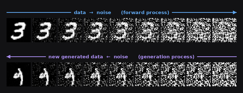
Which makes the third row the instructive one. The reverse SDE and ancestral sampling are the same idea — integrate the stochastic reverse process — and they land at opposite ends of this table, because one of them discretises it well and the other does not. The reverse process is stiff, \(\beta (t)\) diverging as \(t \to 1\), and the Euler–Maruyama arm diverges below \(200\) evaluations (pixel mean \(2.90\) against the data’s \(0.13\), two classes of ten covered) while posting the highest confidence in this section — the previous paragraph’s warning arriving from a second direction. The probability-flow row lags for the same reason, more mildly. So the choice that matters here is not stochastic versus deterministic; it is how the linear part gets integrated, and DDIM does it exactly at either \(\eta \).

The shape carries all the way up: the bestiary DDPM entry below is the same UNet at CIFAR scale, and Stable Diffusion is the same UNet on VAE latents with text cross-attention spliced in. Encoder-decoder-with-skips plus a sampling loop is the whole generative pipeline.

DDPM (Bestiary/Diffusion.lean)

Three new primitives (§ 155, § 156, § 161). The denoiser in Ho et al.’s DDPM (2020, arXiv:2006.11239) is a UNet — literally the same § 155 and § 156 Ronneberger shipped in 2015. Everything “diffusion” lives in the training loop: a forward noise schedule adds Gaussian noise over \(T\) steps, a reverse process learns to predict the added noise, sampling iterates the reverse from pure noise back to a clean image. None of that is a layer. The timestep conditioning MLP (sinusoidal \(\to \) dense \(\to \) dense) is shown as a standalone NetSpec that reuses positionalEncoding from NeRF. Variants: CIFAR config (32x32 backbone), 256x256 high-res config, tiny fixture, timestep embed. Our simplified backbone undercounts vs paper (paper DDPM adds residual blocks, GroupNorm, attention-at-low-res, and per-block time-embedding projection on top of the UNet); the spec’s value is showing the architectural shape, not an exact param match. The lesson is the same one CLIP and NeRF taught: the novelty lives in the training procedure, not in layer design.

def ddpmCifar : NetSpec where
  name   := "DDPM (CIFAR-10, backbone approx)"
  imageH := 32
  imageW := 32
  layers := [
    -- Encoder: 32 → 16 → 8 → 4
    .unetDown 3   128,                            -- 32 → 16
    .unetDown 128 256,                            -- 16 →  8
    .unetDown 256 256,                            --  8 →  4
    .convBn 256 256 3 1 .same,                    -- bottleneck
    .convBn 256 256 3 1 .same,
    -- Decoder: 4 → 8 → 16 → 32
    .unetUp 256 256, .unetUp 256 256, .unetUp 256 128,
    .conv2d 128 3 1 .same .identity               -- predict added noise (3-ch)
  ]

Stable Diffusion (Bestiary/StableDiffusion.lean)

Three new primitives (§ 155, § 156, § 153). The paper that made generative image models consumer-reachable (Rombach et al. 2022, arXiv:2112.10752). Two architectural moves over DDPM, each individually small: (a) latent diffusion — run the diffusion process on 64\(\times \)64\(\times \)4 VAE latents instead of 512\(\times \)512 pixels, cutting spatial work \(\sim \)64\(\times \); (b) text conditioning via cross-attention — at each interior UNet resolution, insert a spatial transformer block that cross-attends from image tokens to CLIP text embeddings. Shown as six separate NetSpecs: VAE encoder, VAE decoder, CLIP text encoder (123M, matches CLIP ViT-L/14 exactly), UNet backbone (190M backbone approx; real SD 1.5 UNet is 865M, missing \(\sim \)675M is the interleaved cross-attention), an explicit spatial-transformer-block spec (uses .transformerDecoder with nQueries = 0 — same primitive Whisper’s decoder uses, same mechanism as DETR’s decoder applied at image-feature resolution), and a tiny end-to-end fixture. Three components are pretrained and frozen during SD’s main training (VAE + text encoder) or constrained-frozen (CLIP); only the UNet trains. SDXL scales the UNet to 2.6B; SD 3 switches the UNet for a DiT transformer. The latent-diffusion plus text-conditioning template is the same.

def sdUNet15 : NetSpec where
  name   := "SD 1.5 UNet denoiser (backbone approx)"
  imageH := 64                                    -- latent resolution, not pixel
  imageW := 64
  layers := [
    .conv2d 4 320 3 .same .identity,              -- stem (latent → channels)
    -- Encoder: 64 → 32 → 16 → 8
    .unetDown 320  640,
    .unetDown 640  1280,
    .unetDown 1280 1280,
    -- Bottleneck at 8×8 (real SD inserts a spatial transformer here)
    .convBn 1280 1280 3 1 .same,
    .convBn 1280 1280 3 1 .same,
    -- Decoder: 8 → 16 → 32 → 64
    .unetUp 1280 1280,
    .unetUp 1280 1280,
    .unetUp 1280 640,
    .conv2d 640 4 3 .same .identity               -- predict noise (4-ch latent)
  ]

10.3.4 Physics — demo: Boltzmann generator on Müller–Brown

Networks whose target is a physical law rather than a labelled set: a Boltzmann density here, a PDE residual, a solution operator and the atmosphere six hours ahead in the entries below. The architectural side is small — an MLP, or a ViT with a Fourier mixer where its attention would be — and the novelty lives in what the model is asked to produce and in what is done with it afterwards.

A Boltzmann generator.

The target is not a dataset. It is a density, \(\exp (-U/kT)\) on the three-well surface Müller and Brown proposed in 1979 as the test case for reaction paths, and the training set is whatever overdamped Langevin manages to produce at \(kT = 20\) in a fixed budget: eight chains of \(10^5\) steps, the Euler–Maruyama integrator the diffusion demo’s table (§ 10.3.3) retired as a sampler, doing its actual job. The network is the 2-D toy demo’s MLP (demos/MainDiffusion2d.lean, \(18{,}178\) parameters, the sincos time channel at \(H = W = 1\)), the loss is that demo’s rank-2 squared-error block, and the flow flag changes one thing in the trainer, the interpolant: \(x_t = (1-t)\, x_0 + t\, \varepsilon \) with target \(\varepsilon - x_0\) (Lipman et al. 2022, arXiv:2210.02747) in place of the cosine-schedule \(x_t\) with target \(\varepsilon \). The sampler is Euler on \(\mathrm{d}x/\mathrm{d}t = v_\theta (x, t)\) from \(t = 1\) to \(0\). Three things change relative to the MNIST demo:

• The ground truth is a formula. \(U\) has a closed form, so the well populations, the mean energy, the free-energy difference between wells and the exact likelihood are all numbers by quadrature on a \(360 \times 360\) grid. Every column of the tables below is exact for the first row.

• A sample set is a free-energy estimate. \(\Delta F_{AB} = -kT \ln (p_A / p_B)\) is read off the populations, and populations are assigned by gradient descent to a minimum rather than by nearest minimum, because the wells are elongated and Voronoi cells put part of A’s basin in C.

• Temperature is a knob the trained model can be moved along without retraining. Every sample carries its own log-density: the Jacobian of each Euler step is two central differences in 2-D, and \(\log |\det (I + h\, \partial v/\partial x)|\) integrated beside the state is the continuity equation for the map actually run. With it, the importance weight \(\exp (-U/kT') / p_\theta (x)\) is a number, and that is the Boltzmann generator of Noé et al. 2019 (Science 365), on an 18k-parameter MLP.

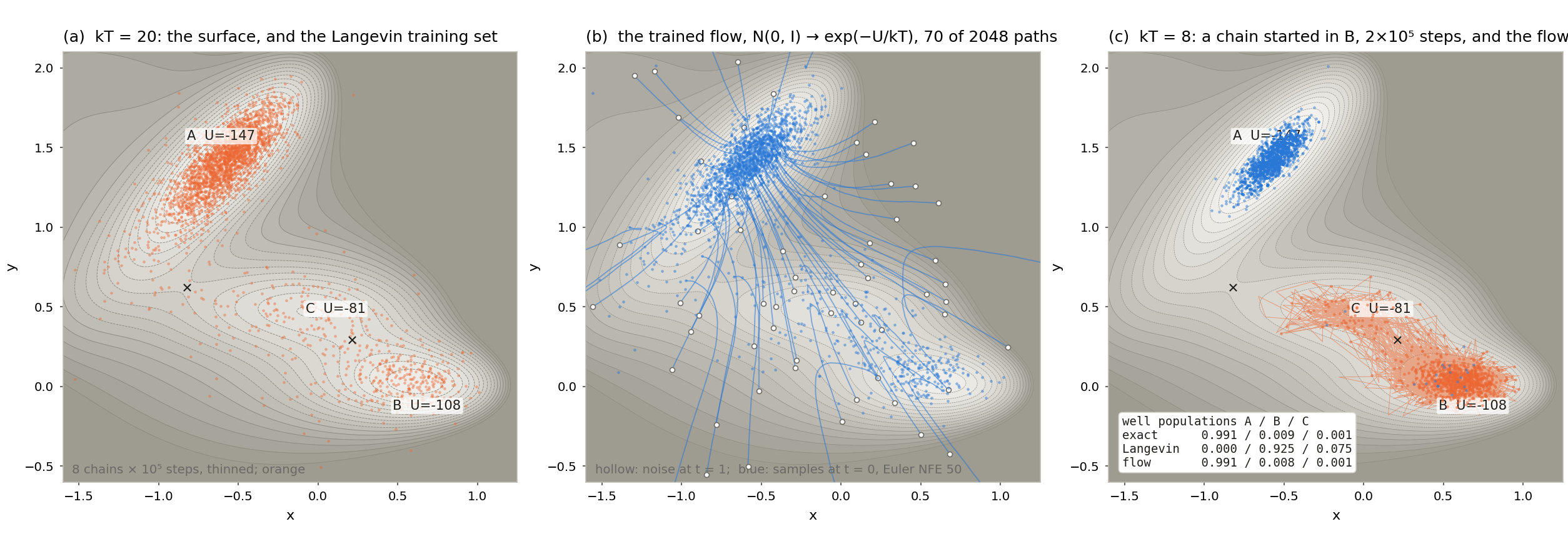
Scored by quadrature, not by eye.

\(kT = 20\), \(2{,}048\) samples per row, the energy distance against an independent exact draw as a multiple of the exact-against-exact floor. The DDPM row is the same network, loss and budget with the cosine-schedule interpolant and DDIM in place of Euler:

The model is faithful to its training set, not to the physics: it over-weights A because the Langevin chains do. Reweighting its own samples by \(p_{20} / p_\theta \) recovers the quadrature row to the last digit. At NFE 2 well B empties while the populations still look plausible, which is why \(\langle U \rangle \) and \(\Delta F\) are columns.

MCMC stalls below the barrier; the generator does not.

The \(kT = 20\) samples reweighted to \(kT' = 12\) and \(8\), naively and with the model’s density in the weight, against a Langevin chain of \(2 \times 10^5\) steps started in well B:

The barrier out of B is 36 units; at \(kT = 8\) the chain never crossed. The naive weights carry the model’s bias in full; with \(1/p_\theta \) in them, samples drawn once at \(kT = 20\) land within 0.3 of quadrature at both temperatures. That is the paper’s claim, and it is the density that makes it.

Straightening the paths.

Rectified flow (Liu, Gong & Liu 2022, arXiv:2209.03003) retrains on the trained flow’s own (noise, sample) pairs; minibatch optimal-transport coupling (Tong et al. 2023, arXiv:2302.00482) pairs each batch’s noise to its data by a minimum-cost assignment. Neither changes the network. Energy distance as a multiple of the floor, with Liu’s straightness at NFE 50:

A one-step generator: after reflow one Euler step lands at \(4.9\times \) the floor where the independent coupling needs ten. The price is the ceiling: both straightened arms plateau above it at NFE 50, because their training set is the first model’s output, biases included.

Boltzmann generator (Bestiary/BoltzmannGenerator.lean)

Zero new primitives for the flow-matching version, one if the original is shown. Noé et al.’s network is RealNVP (Dinh et al. 2017, arXiv:1605.08803): a stack of affine coupling blocks, each splitting the coordinates in half, passing one half through and scaling and shifting the other by two small dense nets of the first. Its log-density is the sum of the log-scales, exact and cheap, and the coupling split is a branch-and-merge the linear NetSpec cannot spell, so the entry shows one conditioner as its own dense net and the block structure in prose, the way the DCGAN entry stands in for transposed convs. The flow-matching version, which is what this book trains, is the demo’s velocity net verbatim; the exact log-density comes from the continuity equation instead of the coupling scales. Variants: the velocity net (18k), one RealNVP conditioner at alanine dipeptide’s width (25k), tiny fixture. The lesson is the one CLIP, NeRF and DDPM taught: the novelty is in what the model is asked to produce — a density, not a picture — and what is done with it afterwards. The architecture is an MLP.

def boltzmannVelocityNet : NetSpec where
  name   := "Boltzmann generator (flow-matching velocity net, Müller-Brown)"
  imageH := 1
  imageW := 1
  layers := [
    .dense 10 128 .relu,        -- 2 coordinates + 8 sincos time channels
    .dense 128 128 .relu,
    .dense 128 2 .identity      -- the velocity ε - x₀, rank-2 MSE block
  ]

Physics-informed neural network (Bestiary/PINN.lean)

Zero new primitives. Raissi, Perdikaris & Karniadakis (2019, J. Comput. Phys. 378; arXiv:1711.10561): the network is a small dense net \(u_\theta (x, t)\) and the loss is the differential equation, its residual evaluated at collocation points by differentiating the network with respect to its own inputs — Burgers’ equation needs \(u_t\), \(u_x\) and \(u_{xx}\) of the net, and the gradient of that residual with respect to the weights is a third-order object. Nothing in the architecture is new; everything in the training signal is. It is an entry and not a demo for that reason: Part 1’s VJP suite differentiates a parameter loss once, and the Boltzmann generator above is the physics this book can train, its physics entering through the target density rather than through derivatives of the network. Variants: the paper’s Burgers net (\(3{,}021\) parameters, the number every reimplementation quotes), Schrödinger (\(4 \times 100\), complex output as two channels), the Navier–Stokes inverse problem (stream function and pressure, two PDE coefficients learned alongside), tiny. \(\tanh \) is modelled as .gelu: the enum has no \(\tanh \), and a ReLU PINN would have \(u_{xx} = 0\) almost everywhere.

def pinnBurgers : NetSpec where
  name   := "PINN (Burgers, 8 x 20 tanh)"
  imageH := 1
  imageW := 1
  layers := [
    .dense 2 20 .gelu,        -- (x, t)
    .dense 20 20 .gelu,
    .dense 20 20 .gelu,
    .dense 20 20 .gelu,
    .dense 20 20 .gelu,
    .dense 20 20 .gelu,
    .dense 20 20 .gelu,
    .dense 20 20 .gelu,
    .dense 20 1 .identity     -- u(x, t)
  ]

Fourier neural operator (Bestiary/FNO.lean)

One new primitive, not shown. Li et al. (2021, arXiv:2010.08895) learn the solution operator of a PDE family rather than one solution: initial condition in, solution out, at any resolution. Four blocks of \(v \mapsto \sigma (Wv + \mathcal{F}^{-1}(R \cdot \mathcal{F} v))\): a pointwise \(1 \times 1\) conv \(W\) beside a spectral convolution that FFTs the field, keeps the lowest \(k\) modes and multiplies each by its own learned complex matrix. The spectral convolution is where the parameters and the idea live, and it is an FFT, a truncation and a per-mode matmul — none of which is a Part 1 layer — so the spec is the non-spectral skeleton (lifting, the four \(W\) bypasses, projection) with the spectral weights counted in prose: the 2-D Navier–Stokes config’s skeleton is \(4{,}577\) parameters and its four \(R\) tensors add \(921{,}600\), so the paper’s \(\sim \)926k model is 99.5 % a layer the linear spec cannot spell. Resolution invariance is that layer’s property alone; the pointwise parts would have it in any architecture. Variants: 2-D Navier–Stokes (width 20, 12 modes), 1-D Burgers (width 64, 16 modes), tiny.

def fno2dNavierStokes : NetSpec where
  name   := "FNO-2d (Navier-Stokes, width 20, 12 modes; non-spectral skeleton)"
  imageH := 64
  imageW := 64
  layers := [
    .conv2d 3 20 1 .same .identity,     -- P: lift (a, x, y) → width
    .conv2d 20 20 1 .same .gelu,        -- Fourier layer 1: W bypass (+ R, 230,400 reals)
    .conv2d 20 20 1 .same .gelu,        -- Fourier layer 2
    .conv2d 20 20 1 .same .gelu,        -- Fourier layer 3
    .conv2d 20 20 1 .same .identity,    -- Fourier layer 4
    .conv2d 20 128 1 .same .gelu,       -- Q: project
    .conv2d 128 1 1 .same .identity     --    → u(x, y)
  ]

FourCastNet (Bestiary/FourCastNet.lean)

One new primitive, shown with the primitive it replaces. Pathak et al. (2022, arXiv:2202.11214) put a ViT on ERA5’s \(0.25^\circ \) grid — \(720 \times 1440\) pixels, 20 variables, \(8 \times 8\) patches, \(16{,}200\) tokens of dimension 768, 12 blocks — and train it to predict the state six hours ahead; rollouts of that map are the forecast. The token mixer is not attention but the adaptive Fourier neural operator (Guibas et al. 2022, arXiv:2111.13587): the FNO’s spectral convolution made data-dependent and block-sparse, \(O(N \log N)\) in tokens where attention is \(O(N^2)\), and at \(16{,}200\) tokens that difference is the model. The spec keeps the patch embedding, dimension, depth and MLP and puts .transformerEncoder where the AFNO block goes, which overcounts: attention at 768 spends \(4 \times 768^2 \approx 2.36\) M parameters a block where AFNO’s block-diagonal complex MLP spends \(0.30\) M; the MLPs, three quarters of a block either way, are the same. Variants: the paper’s model, a \(2^\circ \) version at a size one card trains, tiny.

def fourCastNet : NetSpec where
  name   := "FourCastNet (AFNO-ViT, 0.25°, attention standing in for AFNO)"
  imageH := 720
  imageW := 1440
  layers := [
    .patchEmbed 20 768 8 16200,           -- 20 variables, 8×8 patches → 16,200 tokens
    .transformerEncoder 768 12 3072 12,   -- 12 blocks; the paper's mixer is AFNO
    .dense 768 1280 .identity             -- back to an 8×8×20 patch
  ]

10.3.5 Signal processing — demo: gravitational-wave detection on LIGO strain

Networks whose input is a waveform: strain from an interferometer, raw audio, the spectrogram of a voice. The demo scores a chapter-4 CNN against the detector its field already has, whose performance in Gaussian noise is a closed form; the two entries after it are the audio architectures that read the same kind of input, one sample at a time and one spectrogram frame at a time.

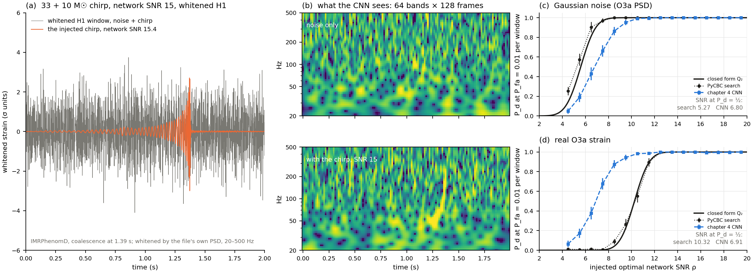
A CNN against the matched filter on LIGO strain.

This demo has a theorem for a ceiling the way blackjack has value iteration and the Boltzmann generator has quadrature. Advanced LIGO’s strain is a time series at audio rates, and a binary-black-hole merger is a chirp that sweeps from 25 to a few hundred Hz in under a second. The Gravitational Wave Open Science Center publishes every observing run under CC BY 4.0 (Abbott et al. 2023, ApJS 267, 29); real events are too few to train on, so the training set is real detector noise with simulated chirps injected at chosen signal-to-noise ratios. The detector to beat is the matched filter: in stationary Gaussian noise it is the Neyman–Pearson optimum, and its detection probability at threshold \(\rho ^\ast \) for a signal of optimal SNR \(\rho \) is a Marcum \(Q\)-function. Three things change relative to the CIFAR demo:

• The data is real detector noise with the signal we chose. Twenty-six file pairs of O3a strain from H1 and L1, science-mode and free of hardware injections, cut into \(2\) s windows and whitened by each file’s own median-Welch PSD over 20–500 Hz. Half the windows carry an IMRPhenomD chirp from PyCBC, masses uniform in \([10, 50]\, M_\odot \), random sky position, projected onto both detectors and scaled to a network SNR uniform in \([4, 20]\). Two noise sets share every window and every injection: Gaussian noise coloured by the same PSD, the theorem’s regime, and the strain itself. \(40{,}760\) training and \(12{,}228\) validation windows.

• The instrument is a closed form, and the filter is checked against it first. PyCBC’s matched filter with the injected template, at the known arrival time, reproduces \(Q_1(\rho , \rho ^\ast )\) on the Gaussian set to within binomial error in every SNR bin — the SNR at half detection is \(4.68\) against the theorem’s \(4.75\) for H1 at a false-alarm rate of \(10^{-2}\) per window — so the injection’s SNR and the whitening agree on one PSD. The search statistic then maximises over the window and the \(\pm 10\) ms inter-detector delay, exactly as a search must, and the CNN, which sees no time, is compared to that.

• The network is Chapter 4’s CIFAR net. CIFAR-CNN8-wide-BN: eight convolutions in four conv-conv-pool stages at 16, 16, 32, 32 channels into the \(2 \times 512\) head. The two edits are the two-channel stem and the two-way output, \(0.83\) M parameters at this input. The input is a \(2 \times 64 \times 128\) image, each channel a constant-Q spectrogram of one detector’s whitened window (64 log-spaced bands over 20–500 Hz, 128 frames); the ordinary train step with integer labels, Adam at \(10^{-3}\) with one warm-up epoch and cosine decay, batch 64, six epochs, under two minutes on one card. Nothing in the codegen moved.

Scored against the theorem.

Detection probability by injected network SNR on the Gaussian set, \(12{,}228\) validation windows, every threshold set on the \(8{,}177\) noise-only windows so that one in a hundred exceeds it. The last column is the SNR at which each row crosses one half:

The filter sits on its closed form and the CNN trails it by \(1.5\) units of SNR. Gabbard et al. 2018 (PRL 120) closed that gap with a one-dimensional network on the whitened strain and ten times the training set; a log-power spectrogram discards the phase the filter integrates, and this is the demo’s number, not the architecture’s ceiling.

Real noise costs the filter, not the network.

LIGO noise is neither stationary nor Gaussian, and the production search adds a \(\chi ^2\) veto for exactly that reason. The same rows on the strain itself, with each model trained on one noise set and scored on both:

Each network is best on the noise it trained on, by a few tenths. The filter loses five units of SNR to glitches at \(10^{-2}\), and at \(10^{-3}\) its threshold is \(417\): eight validation windows hold a glitch that loud, and without a veto the filter has no row. The network trained on Gaussian noise needs an SNR of \(19\) there; the one trained on real strain still reaches half detection at \(7.5\). Training on the real detector is what teaches the glitch tail.

WaveNet (Bestiary/WaveNet.lean)

One new primitive (§ 160). Dilated causal convolutions for raw audio sample prediction (van den Oord et al. 2016, arXiv:1609.03499): exponential receptive field, linear parameter growth. The foundation of neural TTS and PixelCNN. Variants: single stack (0.4M), 3-stack (paper setup, with a NetSpec-linearity approximation), music (single stack, 4.1M), tiny. One honest limitation: the residual-vs-skip dual-output pattern doesn’t linearize cleanly, so the 3-stack variant uses a simplified channel-flow approximation.

def waveNet : NetSpec where
  name   := "WaveNet (single stack, speech)"
  imageH := 16000                                 -- 1 second @ 16 kHz
  imageW := 1
  layers := [
    -- Input embedding: 256 mu-law bins → 32 residual channels
    .conv2d 256 32 1 .same .identity,
    -- One stack of 10 dilated residual blocks (dilations 2⁰..2⁹)
    .waveNetBlock 32 512 10,
    -- Output head: skip-sum → 1×1 → 1×1, 256-way categorical
    .conv2d 512 256 1 .same .relu,
    .conv2d 256 256 1 .same .identity
  ]

Whisper (Bestiary/Whisper.lean)

One new primitive (§ 153). Encoder-decoder transformer over log-mel spectrograms (Radford et al. 2022, arXiv:2212.04356). Encoder is .transformerEncoder on the 1500 post-stem audio tokens; decoder is .transformerDecoder (from DETR) with nQueries = 0 — a clean seq2seq decoder with self-attn + cross-attn + FFN, text tokens coming from a separate .dense vocab\(\to \)D stand-in tied to the LM head. Variants: tiny (7M enc, paper 39M total), base (19M enc, paper 74M), small (85M enc + 153M dec+emb = 238M vs paper 244M), medium (302M enc, paper 769M), large (629M enc, paper 1.55B total), plus a shared decoder spec and tinyWhisper fixture. Encoder and decoder are the same size per variant; adding them together recovers paper totals within 2–3%. The multitask interface (swap a prefix token to change language or switch between transcribe / translate) is prompt-engineering, not architecture — Whisper’s architectural novelty is essentially zero.

def whisperSmall : NetSpec where
  name   := "Whisper small encoder"
  imageH := 1500                                  -- post-stem audio tokens (3000 / 2)
  imageW := 1
  layers := [
    -- 12 encoder blocks, dim 768, 12 heads, mlp 3072
    .transformerEncoder 768 12 3072 12
  ]

10.3.6 Beyond vision — demo: neural quantum states on the Ising chain

Architectures where the task domain is neither a 2D image nor a token sequence: a wavefunction, a radiance field, a shared embedding space. The demo points Chapter 9’s transformer, as an encoder and as a decoder, at a quantum ground state, where there is no dataset at all and the ceiling is a solved model; the entries after it (NeRF, CLIP, LLaVA) make the same point from the other side — several have essentially no architectural novelty, and the interesting work lives in the data, loss, or training procedure.

A transformer as a wavefunction.

Take a ring of \(N\) spins, each up or down. Neighbours want to agree, with strength \(J\); a field \(h\) wants each spin to point sideways, which in quantum mechanics means to be up and down at once. That is the transverse-field Ising chain, \(H = -J \sum _i \sigma ^z_i \sigma ^z_{i+1} - h \sum _i \sigma ^x_i\), and its lowest-energy state is the textbook quantum phase transition: for \(h {\lt} J\) the spins agree, for \(h {\gt} J\) they do not, and at \(h = J\) every pattern in between. The ground state is a probability amplitude \(\psi (\sigma )\) over all \(2^N\) configurations, and a neural quantum state (Carleo & Troyer 2017, Science 355, 602) is a network that maps a configuration \(\sigma \in \{ \pm 1\} ^N\) to its log-amplitude, trained by lowering the energy \(\langle \psi | H | \psi \rangle / \langle \psi | \psi \rangle \). The demo climbs a ladder of three such networks, each written as a closed-form reference times a learned residual, \(\psi _\theta = \psi _{\mathrm{ref}} \cdot \exp f_\theta \), with \(\psi _{\mathrm{ref}}\) the mean-field product state at its optimal angle — a log-amplitude linear in \(\sigma \) that the host adds to the network’s output before any ratio is formed. \(f_\theta \) is an MLP on the \(\pm 1\) spins (\(5{,}057\) parameters at \(N = 12\)); a ViT that reads patches of \(p\) spins as token ids through tokenPositionEmbed, two encoder blocks at \(d = 32\), a mean over tokens and a one-unit head (\(25{,}825\); the transformer wavefunctions of Viteritti, Rende & Becca 2023, arXiv:2211.05504); or a GPT on the same tokens, two causal blocks and an lmHead, whose conditionals are the wavefunction, \(|\psi (\sigma )|^2 = \prod _k p(\mathrm{patch}_k \mid \mathrm{patch}_{{\lt}k})\), so that a sample is an autoregressive draw through the TinyGPT sampling loop with a vocabulary of \(2^p\) (\(25{,}956\); Sharir et al. 2020, arXiv:1902.04057). Three things change relative to the TinyGPT demo:

• There is no dataset. The training signal is the model’s own local energies, \(E_{\mathrm{loc}}(\sigma ) = -J \sum _i \sigma _i \sigma _{i+1} - h \sum _i \psi (\sigma ^{(i)}) / \psi (\sigma )\) with \(\sigma ^{(i)}\) the \(i\)-th spin flipped, so a batch of \(B\) configurations costs one extra forward at batch \(B \cdot N\). The energy is a weighted mean of \(E_{\mathrm{loc}}\) and its gradient, \(\partial _\theta E = 2 \sum _\sigma p_\sigma \, (E_{\mathrm{loc}}(\sigma ) - E)\, \partial _\theta \log \psi (\sigma )\), is one host weight \(w_\sigma \) per configuration. That weight enters the train step through the rank-2 squared-error block of the diffusion demo (§ 10.3.3) with the target set to \(\mathrm{out} - M w / 2\), so the block’s output cotangent is exactly \(w\): the blackjack DQN’s trick (§ 10.4.1) with a physical target, and zero new codegen. At \(N = 12\) the sum runs over all \(4{,}096\) configurations and the gradient is exact; at \(N = 64\) the MLP and ViT sample by Metropolis on \(1{,}024\) chains and the GPT draws independent samples.

• Structure first, the network models the rest. At \(f_\theta = 0\) the ansatz is the mean-field state, so step 0 of every run prints the mean-field energy to six digits and the network only has to learn what mean field gets wrong. For the MLP and ViT the reference is a fixed visible bias; for the GPT it is a fixed bias on the logits, so that the conditionals stay normalised.

• The instrument is a solved model. Every number below is bracketed by a closed form: enumeration of the \(4{,}096 \times 4{,}096\) Hamiltonian at \(N = 12\), and at \(N = 64\) the free-fermion solution of Pfeuty 1970, which agrees with enumeration to \(7 \times 10^{-15}\) where both apply. The variance of \(E_{\mathrm{loc}}\) over the samples is the instrument that needs no ceiling: zero for an eigenstate at any \(N\).

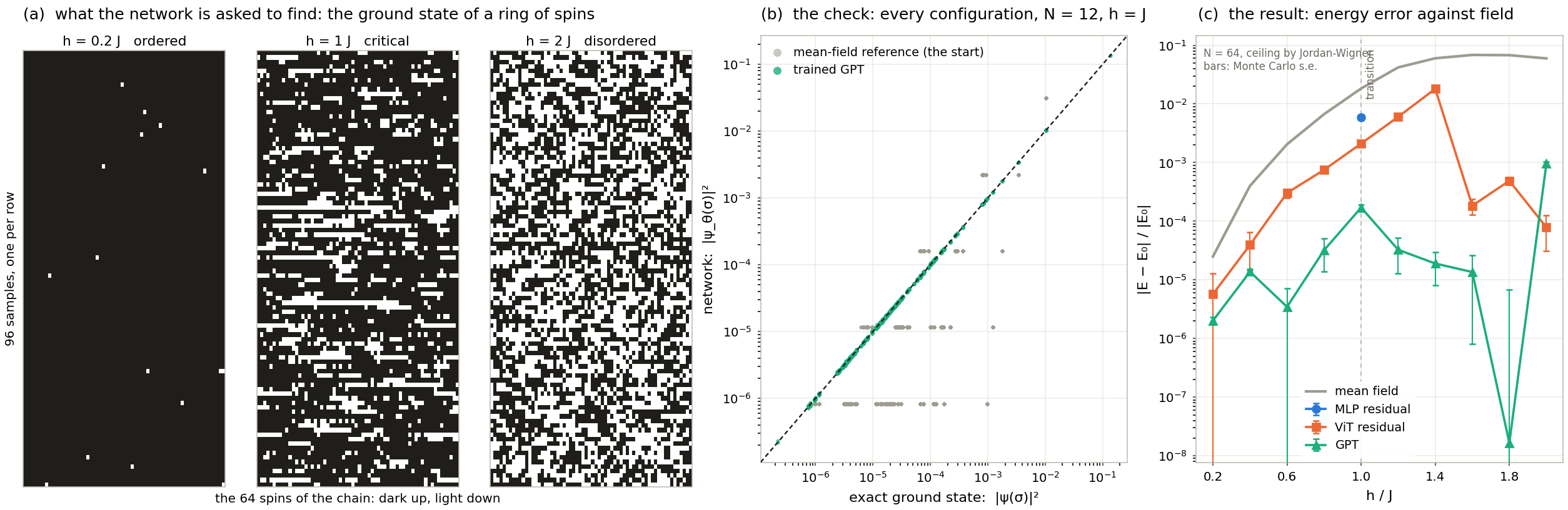
The ladder at the critical point.

\(h = J\), Adam with cosine decay, \(4{,}000\) steps at \(N = 12\) and \(2{,}000\) at \(N = 64\), one RTX 4060 Ti: 50 s to 330 s per row at \(N = 12\) with the XLA compile included and about twenty minutes at \(N = 64\). The \(N = 64\) energies are means over the final \(8{,}192\) samples, whose Monte Carlo standard error is below five percent of every entry:

At \(N = 12\) every rung sits three to four orders below the floor and the GPT, whose conditionals are the wavefunction, is the best of them at every field in the sweep. At \(N = 64\) the ladder separates, and the sampler is why: the GPT’s draws are independent and its gradient noise is only the batch’s, so it holds \(10^{-5}\) to \(10^{-4}\) at every field but the critical point, while the ViT on Metropolis chains is ten to a thousand times worse at the same parameter count and step budget, and at \(h = 1.4\) doubling its chains and steps makes it diverge. That is the regime stochastic reconfiguration (Sorella 1998, PRL 80, 4558) exists for; nothing at \(N = 12\) needed it.

Three things the sweep taught.

The reference decides the small-field rows, and the ablation says by how much: the same ViT, from the uniform state and from the mean-field state, is three orders of magnitude apart at \(h = 0.2J\) (\(3.0 \times 10^{-5}\) against \(1.6 \times 10^{-8}\)), two at \(0.4J\), and level at \(h = J\), where the reference is as wrong as the uniform state and the network does all the work either way. Low variance with a wrong energy is the wrong state: the ViT at \(N = 12\), \(h = 0.8J\) converges to \(5.4 \times 10^{-4}\) with a variance three times lower than its neighbours’, unmoved by seeds, steps, width, depth or patch size, and its excess energy is \(\Delta /2\) to three digits, \(\Delta \) the splitting between the even- and odd-parity states — it converged to the symmetry-broken half of the finite-\(N\) cat state that the product-state reference imprints, and the fix was more structure, not more network: the symmetrised reference \(\psi _{\mathrm{MF}}(\sigma ) + \psi _{\mathrm{MF}}(-\sigma )\), one logaddexp on the host, takes it to \(2.0 \times 10^{-5}\). And signs are the open row. The Ising ground state is positive, so the rungs above are real; the \(J_1\)–\(J_2\) Heisenberg chain is frustrated and its ground state has a sign structure, so the head gets a second slot, \((\log |\psi |, \varphi )\), with Marshall’s sign rule as the reference phase and two host weights per configuration through the same block. At \(N = 16\) the phase head learns the Marshall signs from scratch at \(J_2 = 0\) (fidelity \(0.9985\)), every arm finds the Majumdar–Ghosh dimer state at \(J_2 = J_1/2\) to \(3 \times 10^{-6}\) with fidelity \(1.000\), and past that point, where the rule breaks, every arm stalls at \(10^{-2}\) with a fidelity below \(0.6\) that four times the width and twice the steps move only to \(0.58\).

Two gates sit under the table. The autoregressive sampler, drawn \(16{,}384\) times from a trained \(N = 12\) state and scored by table lookup, lands within \(0.1\) standard errors of the same state’s enumerated energy; on a trained state a single check scatters wider than \(N(0, 1)\) because \(E_{\mathrm{loc}}\) is heavy-tailed, so the pooled test over eight draw seeds is the one that decides. And step 0 of every run is the floor row to six digits, which is the check that the host adds the reference where the ansatz says it does. The trainer is demos/MainNqsIsing.lean; the closed forms, the Lanczos ceiling and every table are scripts/demos/nqs_metrics.py.

NeRF (Bestiary/NeRF.lean)

Two new primitives (§ 161, § 162). The "it’s literally just an MLP" paper (Mildenhall et al. 2020, arXiv:2003.08934). Under 600K params at canonical config; the architectural novelty is nonexistent. What makes NeRF work is the positional encoding + the volumetric-rendering loss — both outside the network, not layers in it. Variants: canonical (593K), fast (167K hidden=128), tiny fixture.

def nerf : NetSpec where
  name   := "NeRF (canonical)"
  imageH := 1
  imageW := 1
  layers := [
    -- Positional encoding of (x,y,z): 3 coords × 2 × 10 freqs = 60-dim
    .positionalEncoding 3 10,
    -- 8-layer MLP with mid-skip + dual density/RGB heads.
    -- encodedDirDim = 3·2·4 = 24 (3D view direction, 4 frequencies)
    .nerfMLP 60 24 256
  ]

CLIP (Bestiary/CLIP.lean)

Zero new primitives. Two textbook encoders glued together by a contrastive loss (Radford et al. 2021, arXiv:2103.00020): a ResNet-50 or ViT-B for images, a 12-layer causal transformer for text, each with a final linear projection to a shared embedding space. Variants: CLIP-RN50, CLIP-ViT-B/32 (151M, paper-exact), CLIP-ViT-L/14 (427M, paper-exact), tiny fixture. The architectural lesson from CLIP is identical to NeRF’s: the novelty lives in data and objective, not in layer design.

def clipViTB32ImageEncoder : NetSpec where
  name   := "CLIP-ViT-B/32 (image encoder)"
  imageH := 224
  imageW := 224
  layers := [
    -- ViT-B/32: patch size 32 → 49 patches, dim 768, 12 blocks, 12 heads
    .patchEmbed 3 768 32 49,
    .transformerEncoder 768 12 3072 12,
    -- [CLS] token → shared 512-dim embedding space
    .dense 768 512 .identity
  ]

LLaVA / LLaVA-1.5 (Bestiary/LLaVA.lean)

Zero new primitives. The cleanest exhibit of the modern vision-language pattern (Liu et al. 2023, arXiv:2304.08485; LLaVA-1.5: arXiv:2310.03744): frozen CLIP ViT encoder + small MLP projector + (mostly) frozen LLaMA/Vicuna language model. Trained in two stages — projector-only pretrain, then joint instruction fine- tune. Shown as separate NetSpecs per component: vision encoder (303M, matching CLIP ViT-L/14), LLaVA-1 single-linear projector (4M), LLaVA-1.5 two-layer MLP projector (21M), LLM backbones at 7B and 13B. The LLM specs undercount real LLaMA by \(\sim \)23% because our .transformerEncoder uses a standard 2-projection FFN while LLaMA uses SwiGLU (3 projections); depth / width / heads still match. Key ratio: the projector is 0.3% of total LLaVA-1.5 7B parameters — the entire interesting work of the model lives in  21M of trainable bolt-on between two pretrained backbones. BLIP-2, Flamingo, and every modern VLM demo generalize this template with fancier adapters (Q-Former, Perceiver resampler, gated xattn-dense), but the frozen-backbone-plus-adapter shape is the same.

def llava15Projector : NetSpec where
  name   := "LLaVA-1.5 projector (2-layer MLP)"
  imageH := 576                                   -- visual token count (24×24)
  imageW := 1
  layers := [
    -- The entire LLaVA architectural contribution: map CLIP's 1024-dim
    -- image tokens into the LLM's 4096-dim embedding space. ~21M params
    -- — roughly 0.3% of total LLaVA-1.5 7B. GELU between is zero-param.
    .dense 1024 4096 .identity,
    .dense 4096 4096 .identity
  ]

10.3.7 Structure — demo: a distogram ResNet against the CASP16 field

Networks whose input is a protein’s sequence and whose output is its shape. The demo is the recipe that held the field from 2018 to 2020 — a deep two-dimensional residual network predicting a histogram of distances for every pair of residues, and a fold obtained by descending that histogram’s negative log-likelihood — with a frozen protein language model in place of the multiple-sequence alignment those methods read, scored on CASP16’s targets beside the groups that predicted them blind. The entry after it is the architecture that ended that era.

A residual network on residue pairs.

A protein is a string over twenty letters, and its fold is set by which residues end up near each other. Write the distance between the \(\beta \)-carbons of residues \(i\) and \(j\) as a histogram over 64 bins from 2 to 22 Å, one per pair: that \(L \times L\) array of histograms is the distogram, and AlphaFold 1 (Senior et al. 2020, Nature 577, 706) and trRosetta (Yang et al. 2020, PNAS 117, 1496) were exactly this shape: per-residue features tiled into an \(L \times L\) pair tensor, a deep 2D ResNet, a histogram per pair, and a fold by gradient descent on the histogram’s negative log-likelihood over coordinates. Those methods read a multiple-sequence alignment; here the per-residue features are the final-layer representation of ESM-2 (Lin et al. 2023, Science 379, 1123), a protein language model trained on sequences alone, frozen, \(2{,}560\) wide at its 3B-parameter size, with the model’s own contact map — a logistic regression on its attention heads — riding along as one pair channel. The input is a single sequence, and the language model runs once, outside the proof. The network is Chapter 5’s ResNet with its strides removed — sixteen of its basic blocks at 128 channels, residualBlock 128 128 16 1 — with one new layer in front (the pair tile, § 157: two dense maps and an outer sum) and a \(1 \times 1\) head of 132 channels — the 66-class distance head, which is the 64 bins, a “beyond 22 Å” class and an “unobserved” class at weight zero, how a missing residue leaves the loss, and trRosetta’s three orientation heads, the dihedrals \(\omega \) and \(\theta \) and the angle \(\varphi \) between the two residues’ \(\mathrm{C}_\alpha \)–\(\mathrm{C}_\beta \) bonds in \(15^\circ \) bins. \(5{,}418{,}244\) parameters. Training reads every protein chain the PDB released before CASP16 opened on 2024-05-01, one representative per 40 % sequence cluster, \(26{,}310\) chains, as random \(96 \times 96\) windows of their pair maps, 100 epochs in 21 hours on one RTX 4060 Ti; inference tiles the same window over a target at stride 32 and averages the logits, so the trained artifact is the one that is scored. The fold is Adam on the smoothed negative log-likelihood of the predicted distances and angles over one pseudo-\(\mathrm{C}_\beta \) point per residue, with a chain term and a clash term, from a classical-MDS start, in both mirror images. Three things change relative to the segmentation demo:

• The input is a pair map built on the host from a frozen model’s output. The pair tile takes the two residue blocks of a crop, \(2 L D\) numbers per example, projects each through its own \(D \to C\) map and outer-sums them into the \([C, L, L]\) map; \(K\) host pair planes are concatenated behind the tile’s channels. It is the one new layer and the one new proof item, Proofs/Foundation/PairTile.lean: the backward in each weight is the cotangent summed over the broadcast axis, then contracted with the block — the two reduce + dot_general pairs the emitter writes — and there is no input gradient, because the blocks are the language model’s and it is not trained. Everything downstream of the tile is the chapter’s; the demo’s gradient evidence is the finite-difference check on the tile’s weights and the eval \(\equiv \) train identity, not a whole-net step tie.

• The loss has four heads and the label is packed. perPixelMultiCE is the segmentation demo’s weighted per-pixel cross-entropy summed over \(K\) heads of one output tensor, the \(K\) labels carried mixed-radix in the one int32 plane the segmentation ABI already passes, each head’s “unobserved” class at weight zero. One sentence the fold needs: lDDT is a distance score and cannot see a mirror image, TM-score superposes with a proper rotation and can, and a fold from distances alone has that ambiguity — the true trace of T1235-D1 and its mirror both score a \(\mathrm{C}_\beta \)-lDDT of 1.00, at TM-scores of 1.00 and 0.34. The \(\omega \) dihedral is chiral, so with the orientation heads the hand is the lower-energy one.

• The instrument is the field. CASP16’s Phase-1 targets — 84 evaluation units whose experimental structures were released after the predictions were in — scored the way CASP scored them: OpenStructure’s lDDT and US-align’s TM-score reproduce the official table to the printed digit on nine field models, and our fold and every group’s model are reduced to the same pseudo-\(\mathrm{C}_\beta \) atom before they are compared. The training set is the information the field had, a date cut; purging the 82 chains homologous to a target is an ablation, and is worth nothing. The single-sequence reference is ESMFold, the same language model under the folding trunk its authors trained for it.

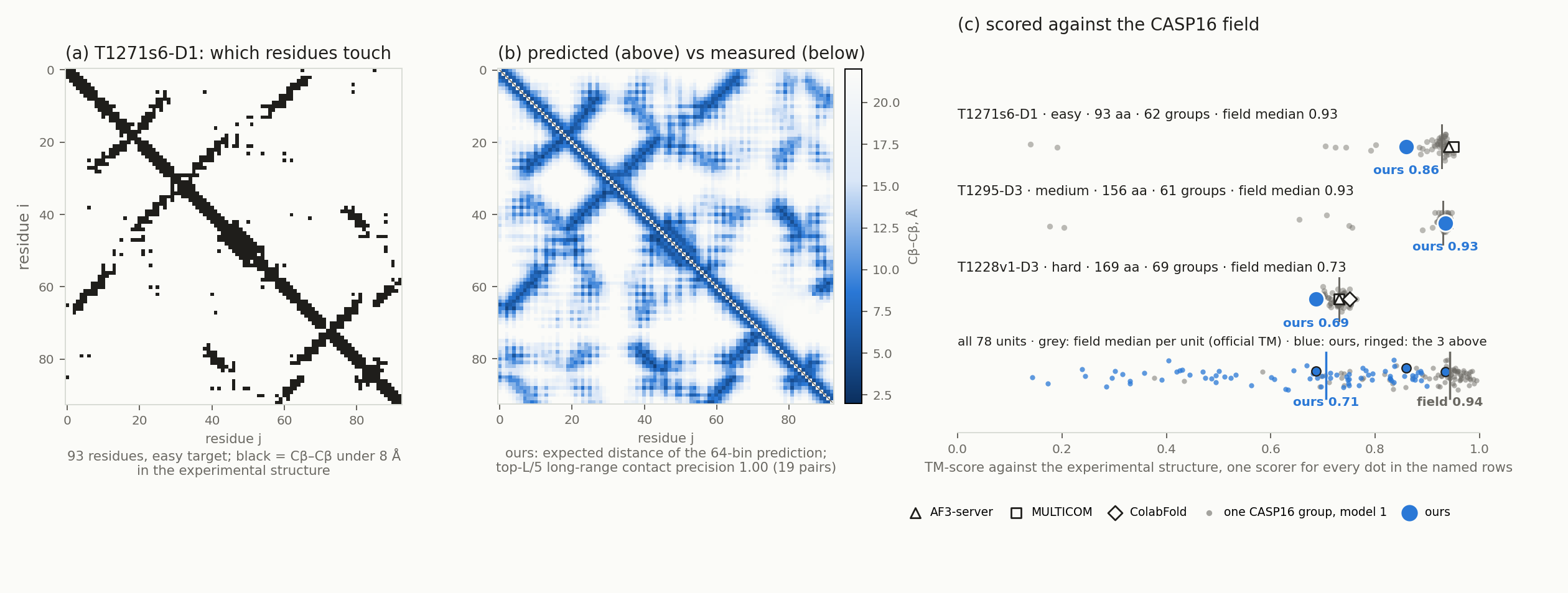
The bracket on the CASP16 targets.

Top-\(L/5\) long-range contact precision over the 84 evaluation units (a long-range pair is 24 or more residues apart; the number is the fraction of the \(L/5\) most confident such pairs that are within 8 Å), the recall of the true long-range contacts at \(P {\gt} 0.5\), and the fold’s \(\mathrm{C}_\beta \)-lDDT and TM-score over the 78 units the fold and the field both cover:

The language model is the lever and the ladder says by how much: at 64 channels and 30 epochs the precision runs \(0.585 \to 0.735 \to 0.838 \to 0.840\) from ESM-2’s 35M to its 150M, 650M and 3B sizes, each model’s own contact head \(0.474 \to 0.623 \to 0.754 \to 0.759\) beneath it, so the network adds 0.08 to 0.11 on every language model and the ladder is flat on precision past 650M, where the 3B step shows in the fold (\(+0.012\)). On top of 650M each of width (128 channels), a 96-residue crop and the model’s contact map as a pair channel is worth \(+0.01\) to \(+0.02\) of precision and the three add, the plane giving the hard class the most (\(+0.09\) on its own); with the 3B features they reach \(0.880 / 0.622 / 0.632\) at 30 epochs, and the orientation heads cost 0.003 of precision and buy \(+0.013\) of TM-score through the \(\omega /\varphi \) restraints. The book run is that configuration at 100 epochs, and the schedule bought nothing: against its 30-epoch twin (\(0.877 / 0.628 / 0.645\)) the paired differences over units are \(-0.004\), \(-0.001\) and \(+0.001\) with every 95 % interval across zero, and validation precision is level from epoch 20. A second seed moves any arm by at most 0.002 on any column, an ensemble of five arms does not beat its best member, and the fold is converged: under its own potential the experimental trace has higher energy than our fold on 78 of 78 units, the map’s own mean distances score an lDDT of 0.615 against the fold’s 0.627, and the two correlate at 0.90, so what the fold realises is the map.

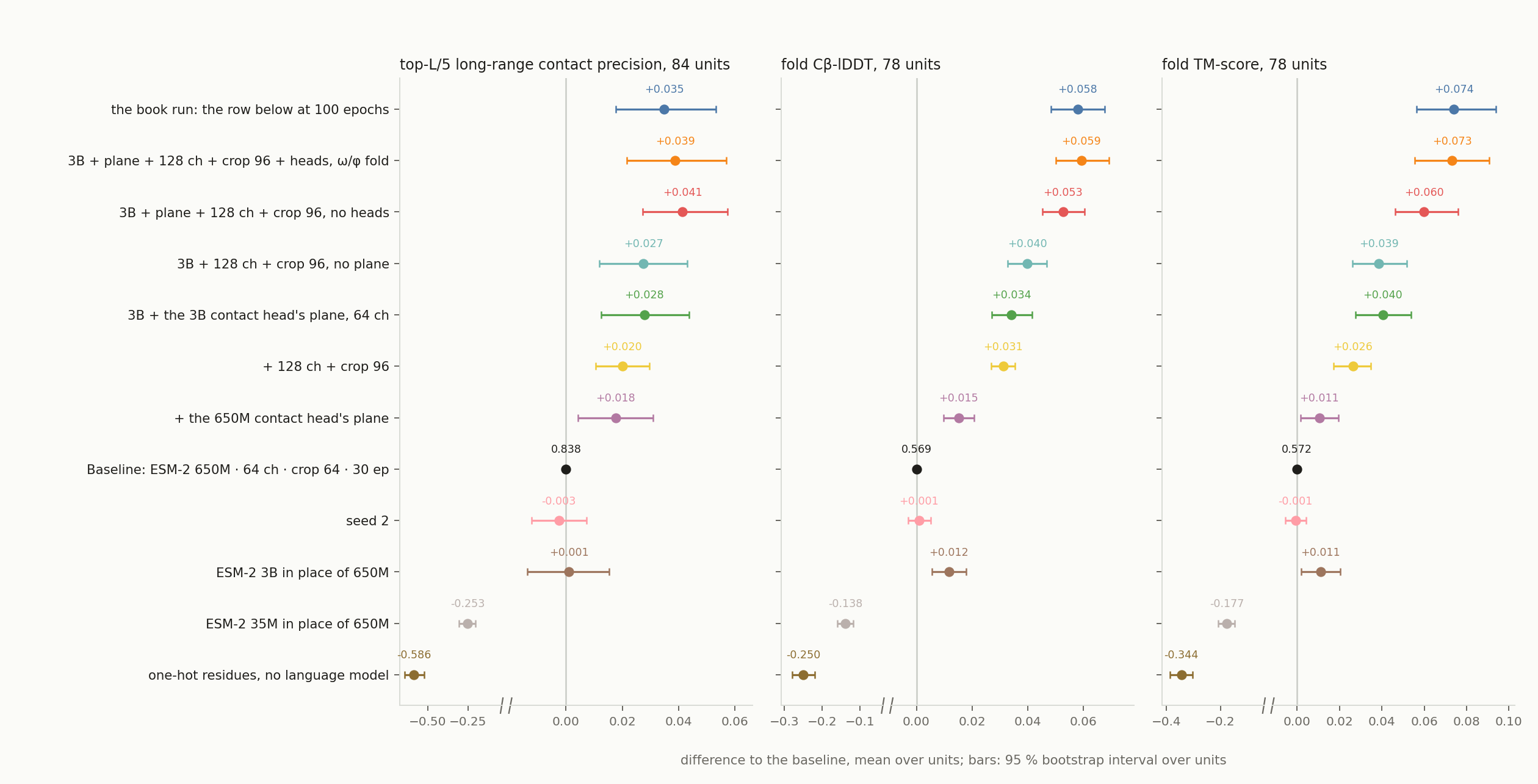
The gap is the story. Our TM-score of 0.646 sits at the field’s third percentile; the median first model is 0.892 over the same 78 units, \(0.945 / 0.883 / 0.656\) on the easy, medium and hard classes against our \(0.716 / 0.617 / 0.495\), and OpenComplex, the lowest of the thirty groups that predicted all 78, is at 0.768. Two readings, from the units themselves. Sixteen units have top-\(L/5\) precision under 0.85 and fold to 0.34 where the field’s median is 0.83 — four of them “easy”, which in CASP’s vocabulary means a template exists in the PDB, something a single-sequence model cannot see — and they are two fifths of the distance; the other 62 fold to 0.72 against 0.91, and there the top \(L/5\) pairs are right, the next \(L\) are half wrong and the recall at \(P {\gt} 0.5\) is 0.49. ESMFold places the two halves: the same language model under the trunk and structure module its authors trained for it folds the 78 to \(0.751 / 0.778\), \(+0.132\) of TM-score over our head with a 95 % interval of \([+0.103, +0.167]\) and better on 71, 0.84 against 0.72 on the 62 units where our top contacts are right and 0.53 against 0.34 on the 16 where they are not. So the head is the larger half of the gap and the input is the other: an alignment is what the field’s models read and ESMFold does not, and half of the sixteen are blind to the language model too.

What this is not: a 5.4M-parameter network on a single sequence, 65 residues of receptive field in a 96-residue window, folded as one point per residue. The field’s models read alignments and templates and build an all-atom chain through a structure module; the architecture that does so is the entry below, and AlphaFold 2’s distogram head is this demo’s network grown into a 48-block pair stack with the alignment beside it.

Four gates sit under the table. The scorer reproduces CASP16’s official lDDT and TM-score to the printed digit on nine field models — AF3-server, MULTICOM and ColabFold on three targets — and GDT_TS within a point. Folding a target’s true distogram recovers its structure (TM-score 0.9999 on T1235-D1) and the mirror scores 0.34. The packed training pools are checked against the per-chain files before any run, and a 64-chain memorization probe must leave the separation prior. And lake exe distogram-casp smoke finite-differences the emitted gradient of the pair tile’s weights, a body weight and each head’s bias against the step’s own first Adam moment, and checks that the evaluation forward’s loss at one batch’s statistics is the training step’s. The trainer is demos/MainDistogramCasp.lean; the chain list, labels, embeddings and packing are scripts/datasets/casp16_*.py, the fold, scoring, table and figures scripts/demos/casp16_*.py.

AlphaFold 2 Evoformer (Bestiary/Evoformer.lean)

Two new primitives (§ 163, § 164). Dual-representation (MSA + pair) doesn’t fit a linear NetSpec cleanly; the bestiary shows the two bundled primitives and notes the limitation (Jumper et al. 2021, Nature). Variants: full (76M), mini, tiny.

def alphaFold2 : NetSpec where
  name   := "AlphaFold 2 (Evoformer + StructureModule)"
  imageH := 384                                   -- max residues (N_res)
  imageW := 1
  layers := [
    -- 48 blocks of dual-representation processing (MSA + pair).
    -- Each block bundles: MSA row-attn (w/ pair bias), MSA col-attn,
    -- MSA transition, outer-product mean → pair, triangle-mul updates
    -- (out + in), triangle self-attention (start + end), pair transition.
    .evoformerBlock 256 128 48,
    -- Structure Module: 8 recurrent IPA rounds (weights shared).
    .structureModule 384 128 8
  ]

The two primitives are conceptually separate networks chained back to back; the linear NetSpec flattens that.

Evoformer (48 blocks) is the perception/refinement stage. It maintains a dual representation: a multiple-sequence-alignment tensor \(\mathrm{MSA}\! \in \! \mathbb {R}^{s \times r \times c_m}\) (where \(s\) is the number of homologs found by the database search and \(r\) is the number of residues) and a pair tensor \(\mathrm{Pair}\! \in \! \mathbb {R}^{r \times r \times c_z}\) encoding predicted residue-residue relationships. Each block updates both via seven stacked operations (row attention with pair bias, column attention, MSA transition, outer-product-mean into pair, two triangle multiplicative updates, two triangle attentions, pair transition). Forty-eight rounds of that turn raw evolutionary signal into a self-consistent geometry-implied pair representation.

Structure Module (8 recurrent rounds, shared weights) is the geometry stage. It consumes the final pair tensor + a per-residue “single” embedding and emits 3D backbone frames plus side-chain \(\chi \) angles. Each round runs Invariant Point Attention (IPA) over the residues, updates each residue’s local frame relative to its neighbors, and feeds back into the next round. The shared-weights recurrence is unusual — most networks unroll different parameters per layer — and reflects that each round is the same fixed-point iteration on the protein’s 3D structure.

The bundled-primitive shortcut means Lean sees one NetSpec with two layers; the actual graph is a much larger DAG with the dual representation and the cross-stage handoff. § 163 and § 164 document the bundling explicitly.

10.4 Bestiary entries: game theory

Four games written in Lean, each with its own exact instrument, on one loop: the reward is the game’s, the data is manufactured by playing it, the target is the model’s own later estimate, and the ceiling is exact where the game allows it — blackjack’s by value iteration over its 200 states, poker’s by the best response to the trained strategy, tic-tac-toe’s by the solved game — and, for Pong, a twin fed the six numbers the renderer draws from. The ladder runs tabular Q, then a DQN on a table’s worth of states, then the same DQN from pixels, then regret minimisation under hidden information, then self-play and tree search; every trained rung goes through the squared-error block of the diffusion demo with a host-built target, and none of it is new codegen. The catalogue beside the demos is the AlphaGo family and Deep CFR, the same loops at the scale that made them famous.

10.4.1 Blackjack — DQN against value iteration

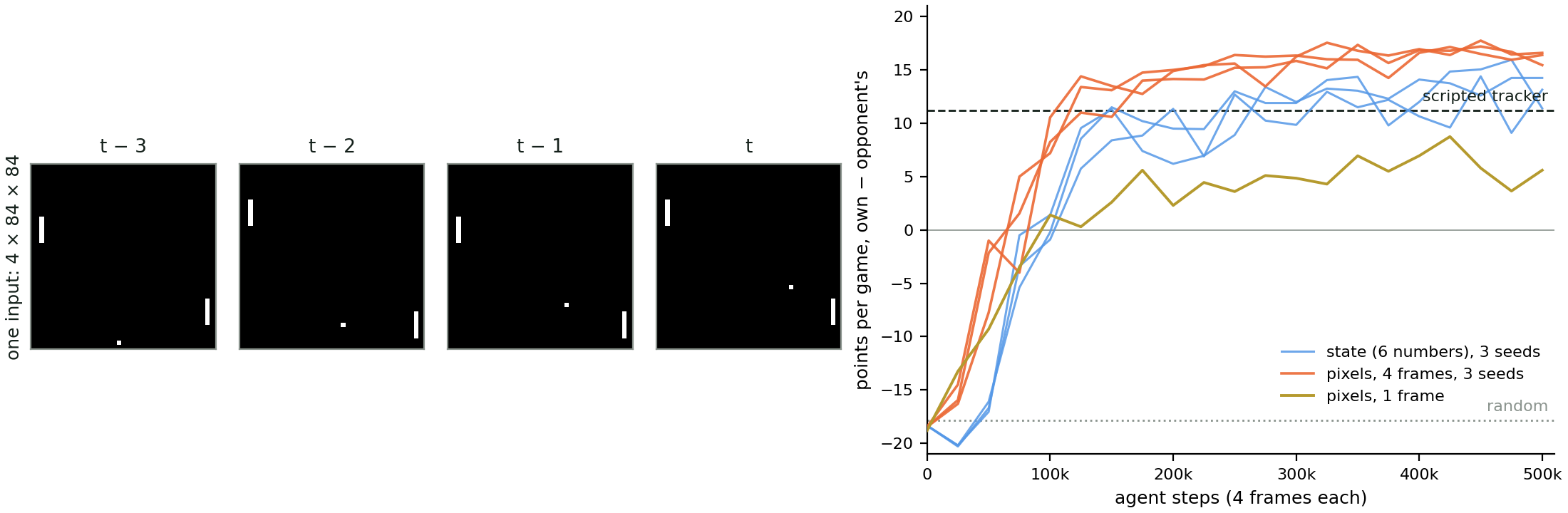
DQN on blackjack.

The demos/MainBlackjackDqn.lean trainer is Mnih et al.’s DQN (2015, Nature) on the blackjack of Sutton & Barto’s Example 5.1, the game written in Lean (LeanMlir/Blackjack.lean) with its RNG threaded through so every hand replays from a seed. The Q-function is a three-layer .dense net on a 29-float one-hot of the observation (player total, dealer’s card, usable ace), \(6{,}210\) parameters. Three things change relative to everything trained so far:

• There is no dataset. Transitions come from playing the game \(\varepsilon \)-greedily against the current network and are kept in a replay ring of 20k; each gradient step samples 128 of them. The book’s other demos read their data from disk; this one manufactures it.

• The target is the model’s own prediction, one step later. \(y_a = r + \gamma \max _{a'} Q_{\text{target}}(s', a')\), with the target network a copy of the online parameters refreshed every 500 updates. The loss is the squared-error block the DDPM demo trains with (§ 10.3.3): the host runs the eval graph on the batch, writes \(y = Q(s,\cdot )\), overwrites the taken action’s slot with the Bellman target, and hands \(y\) in. The gradient is then zero on the untaken slot and a per-sample TD error on the taken one. Zero new codegen.

• The instrument is a solved game. Blackjack under these rules is a 200-state, two-action MDP with known odds, so value iteration gives the optimal policy and the exact mean reward of any policy, in milliseconds. Every thousand updates the greedy policy is read off the network over all 280 observations in one batched forward and scored exactly. The ceiling of the training curve is a theorem about the rules, not a number somebody measured.

Every arm scored against the theorem.

Mean reward per hand; exact by value iteration, Monte Carlo over \(10^6\) hands with its standard error, and agreement with the optimum over the 200 decision states. The two value columns agree within two standard errors on every row, which is the check that the simulator and the DP describe the same game:

The published table is the strategy card the first book shipped as its ceiling. It sits four cents a hand below the optimum because it is for a different game — doubling, splitting and a dealer who plays differently — and it ignores the usable ace entirely. Tabular Q needs a visit-count step size to get past \(177/200\); a constant one chases the moving bootstrap target forever. Figure 10.14 is the policy itself, cell by cell.

The DQN’s own table.

One seed per arm, exact value at the end of training; the gate is the DQN within \(0.01\) of tabular Q’s exact value, which every 200k-update arm passes:

Double DQN (van Hasselt et al. 2016, arXiv:1509.06461: argmax from the online net, value from the target) is the best of the four, and the learning-rate decay does nothing, because the late-training jitter is not in the step size: it is the greedy readout flipping knife-edge cells whose two actions are worth the same to three decimals. The 1000-update readouts move by \(\pm 0.005\) late in every arm, so the gap between the first two 200k rows is inside that. Ten minutes on one card at 6% utilisation, each.

10.4.2 Pong — DQN from pixels against the six-number state

demos/MainPongDqn.lean is the same loop on a Pong written in Lean (LeanMlir/Pong.lean: an \(84 \times 84\) field, two-pixel paddles, frame skip 4, a scripted opponent that tracks the ball at 1.5 pixels a frame after a four-frame delay, a game to 21, deterministic from a seed, five million raw frames a second with no emulator and no ROM), under Mnih et al.’s 2015 recipe: a replay of 100k transitions, \(\varepsilon \) from 1 to 0.1 over the first 100k agent steps, a target network copied every 1,000 updates, one gradient step per four agent steps, batch 32, Adam at \(10^{-4}\), \(\gamma = 0.99\), 500k agent steps — two million frames. The Bellman target goes into the taken action’s slot of the squared-error block exactly as in blackjack. Two things change: the observation is an image, so the Q-function is Chapter 3’s CNN kit at \(84 \times 84\) (three convolutions with pooling standing in for the paper’s strides, a dense 512, three outputs; 1.7M parameters), and one frame does not contain the ball’s velocity, so the input is a stack of the last four. The bracket is built into the game: the same DQN on the six numbers the renderer draws from — ball position and velocity, the two paddles — is a twin that is handed everything the pixels could carry, the scripted opponent is the bar, and a one-frame input is the ablation.

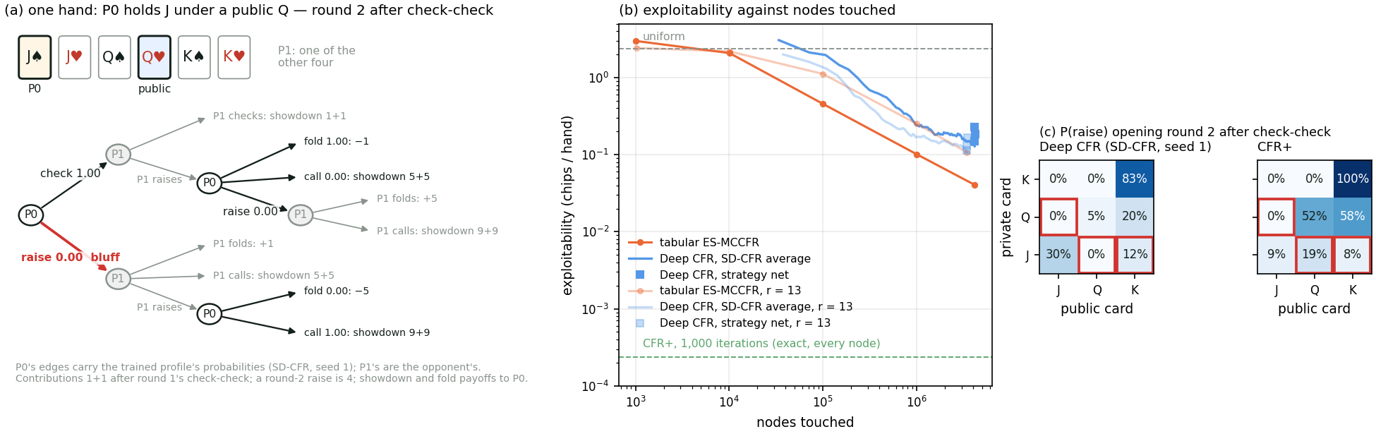
Every arm against the scripted opponent.

Mean points per game over twenty fresh games after training, with the standard error; the baselines over a hundred games (lake exe pong-env 100):

One frame cannot see velocity, and the row says by how much: \(+4.6\) against \(+15.5\), the gap between a paddle that reaches the ball and one that guesses. The state twin was meant to be the ceiling and is not: the pixel network sits above it on every seed (\(+15.47\) against \(+13.45\) on average) and at every opponent speed (1.0 / 1.5 / 2.0 pixels a frame: state \(+14.45\) / \(+13.45\) / \(+9.80\), pixels \(+17.75\) / \(+15.60\) / \(+14.45\)). The six numbers are all the pixels could carry, so the gap is in what each network learns from its input, and it is not dissected here. An update was 24 milliseconds, twenty of them the shim re-pushing 20 MB of parameters and Adam moments every step; with that state resident on the device (trainStepAdamF32DdpmR) it is 14.6, and a pixel run 27 minutes on one card.

10.4.3 Poker — Deep CFR against the exact best response

demos/MainDeepCfrLeduc.lean is Brown, Lerer, Gross and Sandholm’s loop (Deep CFR, ICML 2019, arXiv:1811.00164) on Leduc hold’em written in Lean (LeanMlir/Leduc.lean): a two-player, fixed-limit, one-card poker — \(r\) ranks in two suits, three for the classic jack–queen–king deck, an ante of one, two betting rounds with bets of two then four and at most two raises each, one public card between the rounds, a pair beats a higher rank — and the first game in this section with hidden information. The answer is therefore not a move but a mixed strategy: an equilibrium raises a jack it knows is losing about a fifth of the time, because a player who never bluffs can be read. Each iteration and player, one batched forward of the player’s advantage network over every information set gives the current strategy as a table (regret matching on the positive advantages), a thousand external-sampling traversals in C write instantaneous regrets to the player’s advantage reservoir and the opponent’s strategy to a strategy reservoir (reservoir sampling, a million rows each), and the advantage network is re-initialised and retrained from scratch on its reservoir, a thousand Adam steps at batch 512. After a hundred iterations the strategy network is trained on the strategy reservoir; Single Deep CFR (Steinberger 2019, arXiv:1901.07621) comes for free, the exact average of the hundred stored profiles weighted by iteration and by each profile’s own reach, no strategy network. The network is the Leduc papers’ three dense layers of 64 (Bestiary/DeepCFR.lean, 10.5k parameters, no BatchNorm), and the loss — a weighted squared error on the legal slots — goes through the squared-error block as a host-built target, tic-tac-toe’s move. Two things change relative to the three games around it:

• The instrument is the best response, and it is exact. Suits never matter in Leduc (there are no flushes), so the game is solved at rank level — \(6r + 30r^2\) information sets, 288 at \(r = 3\) against OpenSpiel’s 936 suit-aware ones, which fold onto them one-to-one — by vector-form CFR over the public tree with an \(r \times r\) matrix of private ranks at each node: the best response, exploitability (the best responder’s winnings per hand averaged over the two seats, OpenSpiel’s convention), head-to-head and CFR+ to a thousand iterations are 25 milliseconds at \(r = 3\) and under a second at \(r = 13\). Zero is Nash; CFR+ reaches \(2.4 \times 10^{-4}\). Before anything trains, the Lean game is checked against the C tree on every terminal history and both against OpenSpiel’s leduc_poker: every payoff on OpenSpiel’s own histories, and our tables scored by OpenSpiel’s exploitability to \(10^{-6}\) (scripts/demos/leduc_gate0_openspiel.py).

• The sampled table is the bracket, at the same budget. A table is enough at every \(r\) here, so the comparison is the Deep CFR paper’s own axis: exploitability against nodes touched, external-sampling MCCFR on a table against the network, at \(r = 3\), 6 and 13. The trainer’s own traversal with a lookup table in the network’s place must reproduce that curve before the network is trusted (mode=tabular), and does.

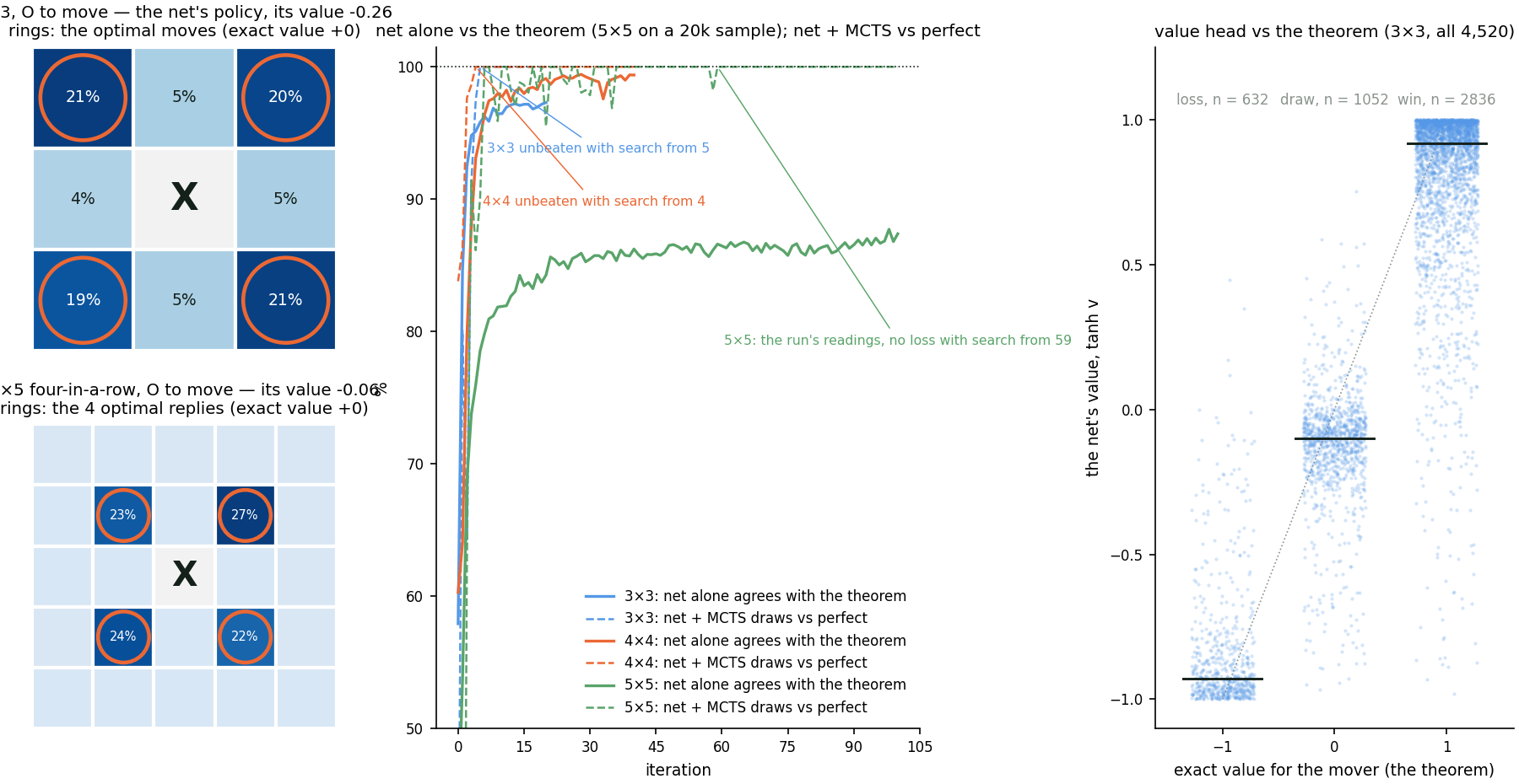
Every arm against the best response.

Exploitability in chips per hand (ante one; a thousandth of a chip is a milli-ante per game, the Leduc papers’ unit) and head-to-head against CFR+ averaged over the two seats. The scripted honest arm raises a pair or a king and folds a jack to a bet; the price-of-honesty arm is CFR+ with its worst-hand raises moved to call; the two Deep CFR rows and the sampled table are at the same 4.1M nodes, three seeds each. The last column is the bluff, the raise frequency opening round 2 with a jack under a queen:

Six minutes a seed on one card. Deep CFR’s exploitability falls from 1.4 at iteration 5 to 0.11–0.15 at a hundred and ends under the honest arm and under the equilibrium with its bluffs removed; at a hundred iterations it is where the Single Deep CFR paper’s Leduc curves are (150–200 milli-antes per game read from its Figure 1a, at 1,500 traversals an iteration to our thousand). It does not beat a sampled table at the same budget on the classic deck: the table is three times less exploitable at 4.1M nodes. The scale arm is where that turns. The same recipe at \(r = 6\) (1,116 sets) and \(r = 13\) (5,148): SD-CFR 0.112 / 0.123 / 0.113 against the table’s 0.053 / 0.066 / 0.058 at 3.6M nodes, then 0.099 / 0.120 / 0.106 against 0.113 / 0.107 / 0.102 at 3.4M — the table’s lead is \(3.1\times \), \(2.0\times \), \(1.0\times \), and at \(r = 13\) the network is the better head-to-head (\(-0.028\) against \(-0.035\) a hand). The table visits all but a set or two at these budgets, so the mechanism is not what it never saw; its estimate of each set is noisier as the sets multiply at a fixed budget, and the network’s error does not grow with them. The bluff column is the finding a reader can check on the figure: the trained profile that is 0.13 exploitable raises the losing jack under a queen 0% of the time where the equilibrium raises it 19.5% (18.6–19.5% over two solvers and three initialisations — the frequency is pinned at \(r = 3\), and is not at \(r = 13\), where the same cell ranges over tens of points), and it bluffs elsewhere instead, a jack under a king 12%. Honesty’s price is exact: moving the equilibrium’s worst-hand raises to call costs 0.186 of exploitability.

What this is not: a two-player, fixed-limit, one-card game, solved at rank level. The scale of the Deep CFR paper is heads-up flop and limit hold’em, where no exact best response exists to score against and the paper’s numbers are against abstractions and head-to-head; no-limit and multi-way poker (Pluribus) are another scale again, and exploitability is not computable there.

10.4.4 Tic-tac-toe — AlphaZero against the solved game

The demos/MainAlphaZeroTtt.lean trainer is Silver et al.’s self-play loop (AlphaGo Zero, 2017, Nature; AlphaZero, 2018, Science) on tic-tac-toe written in Lean (LeanMlir/TicTacToe.lean), \(n \times n\) with \(k\) in a row, \(n\) the one knob. Each iteration plays 256 games in lockstep: at every move a PUCT search of 25 (\(3 \times 3\)) or 100 (\(4 \times 4\)) simulations over the network’s priors and value, one batched forward over the games’ pending leaves per simulation, Dirichlet noise at the root, the move drawn from the visit counts; the visit distribution \(\pi \) and the outcome \(z\) are the targets, and the next iteration plays with the new network. The network is AlphaGo’s plain convolution + ReLU stack (Bestiary/AlphaGo.lean) at tic-tac-toe width, with the policy and value heads merged into one dense output of \(n^2 + 1\) slots: 78k parameters at \(3 \times 3\), 155k at \(4 \times 4\). Three things change relative to the two DQNs:

• The loss has two heads and the codegen has one. The paper’s \((z - v)^2 - \pi ^{\top } \log p\) goes through the squared-error block blackjack’s Bellman target went through: the host runs the eval graph on the batch and writes \(y = \mathrm{out} - \tfrac {n_{\mathrm{out}}}{2}\, g\), with \(g = \mathrm{softmax}(p) - \pi \) on the \(n^2\) policy slots and \((\tanh v - z)(1 - \tanh ^2 v)\) on the value slot, so the block’s gradient is \(g / B\) exactly — the gradient of the batch-mean AlphaZero loss. Zero new codegen, the move the neural-quantum-state demo (§ 10.3.6) makes with its energy gradient.

• Not the bestiary’s tower. The first run used Bestiary/AlphaZero.lean’s convolution–BatchNorm–residual body and diverged at iteration 11. BatchNorm’s batch statistics over nine binary cells are a liability, and with BatchNorm the eval forward the loss reads and the train step’s forward are different functions. Blackjack and Pong made the same choice for the same reason.

• The instrument is the solved game. A position is a base-3 number over the cells, so a memoised minimax fills one byte per index with the exact value and the optimal-move set of every reachable position — 5,478 at \(3 \times 3\), 9,722,011 at \(4 \times 4\). The network alone is scored by the argmax of its masked logits over every reachable decision position (4,520 and 9,062,619), its value head against the exact value, and its match play against a perfect player that draws uniformly from the optimal set. Nothing in the table is sampled but the games.

Five by five, four in a row.

No table exists there (\(3^{25}\) bytes), so the instrument becomes an exact solver — alpha-beta with a transposition table over symmetry-canonical positions — checked against the dense table on every reachable \(3 \times 3\) and \(4 \times 4\) position before it is trusted where no table exists. It establishes that \((5, 5, 4)\) is a draw, and something a reader can check on the figure: after X takes the centre, O’s only drawing replies are the four diagonal neighbours. Two things change in what the table can say: the sweep is a fixed sample of 20,000 random-play decision positions with at least six stones, exact per position but not exhaustive; and the perfect player draws its first move uniformly from the optimal set and plays the solver’s principal move from there.

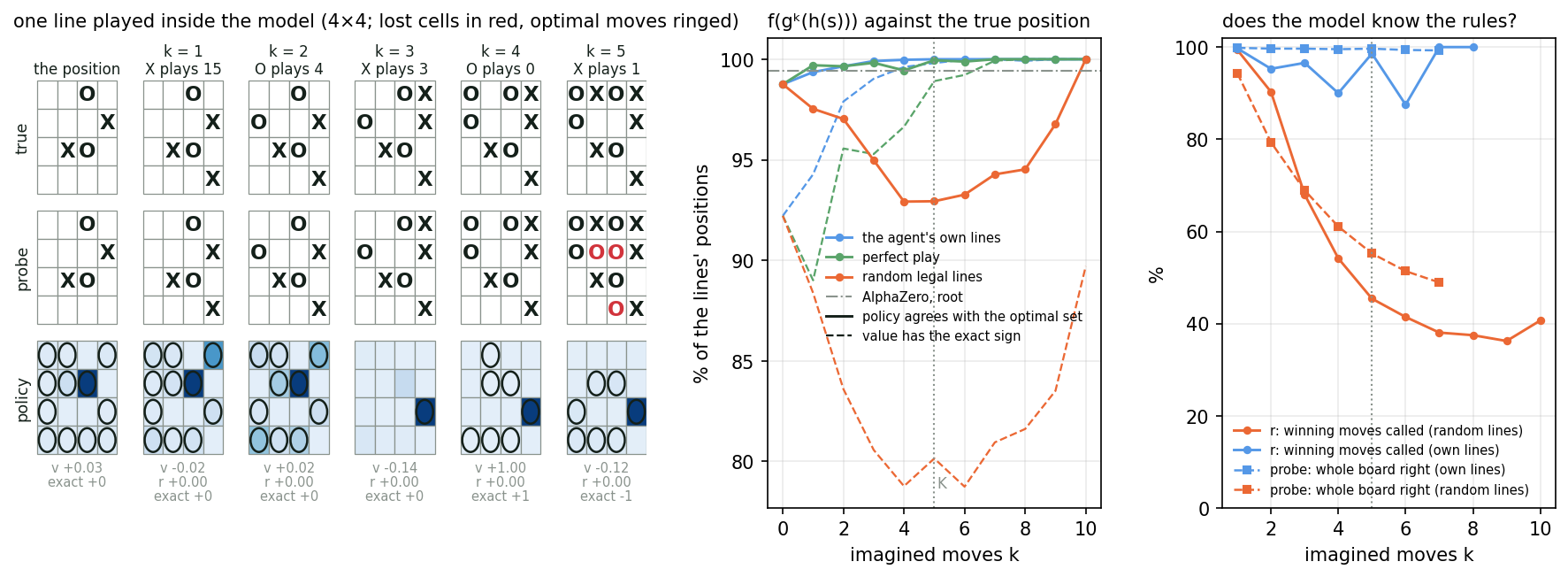
Every arm against the solved game.

Agreement of the arm’s move with the optimal set — over every decision position at \(3 \times 3\) and \(4 \times 4\), over the 20,000-position sample at \(5 \times 5\); the scripted players’ is their expected agreement — and W/D/L against the perfect player as X and as O: 1,000 games each way for the scripted rows (200 at \(5 \times 5\)), and for the network’s rows three independent evaluations of the saved network, 256 games each, pooled:

Twenty iterations and 2.5 minutes on one card at \(3 \times 3\); forty iterations and 10.0 minutes at \(4 \times 4\), the same binary with n=4 — the Python implementation this loop follows (Nair, alpha-zero-general) was expected to take a day on that board. The untrained network’s sweep is the random player’s. Self-play visits 1.2% of the \(4 \times 4\) decision positions and the sweep scores all of them; the misses are mostly forced wins not taken, late in games a competent opponent never produces, and the search closes them — with 25 or 100 simulations the network is unbeaten from iteration 5 and 4, before the network alone is. The value head estimates self-play rather than the theorem (the figure’s right panel): the root ends X-favoured at \(3 \times 3\) because self-play under root noise is. At \(5 \times 5\) the same binary with n=5 k=4 runs a hundred iterations at 400 simulations in 64 minutes. As X the network never loses, alone or with search; as O it still does — 60 games in 768 alone, 23 with search — and its 87.4% on the random-play sample is 92.1% over the exhaustive opening, every position with at most three stones: it is best where the theory is. On this board the search is what closes the second player’s games, and it has not closed them yet.

The entries below are the same loop at the scale that made it famous: the network is a residual tower, the game is Go or chess, and the target is still the model’s own later estimate.

Deep CFR (Bestiary/DeepCFR.lean)

Zero new primitives. Counterfactual regret minimisation with the two tables replaced by networks (Brown, Lerer, Gross and Sandholm 2019): an advantage network per player regresses the sampled counterfactual regrets of an information set and regret matching on its positive outputs is the current strategy; an average-strategy network regresses the strategies played, or, in Single Deep CFR (Steinberger 2019), the stored advantage networks are averaged exactly instead. The paper’s network is two branches — summed card embeddings through three dense layers, bet flags and sizes through two — concatenated into three more with skips where the widths agree and a normalisation of the last layer’s features, 98,948 parameters for heads-up flop hold’em; its Leduc experiments and ours use three dense layers of 64. The architecture is not the point and the paper says so; the loop is, and § 10.4.3 trains it.

def deepCfrLeducNet (r : Nat := 3) : NetSpec where
  name   := s!"Deep CFR Leduc r{r}"
  imageH := 1
  imageW := 1
  layers := [
    -- 2r + 24 features: one-hot cards with rank scalars, pair and
    -- above-public flags, the betting history, the round, the pot.
    .dense (2 * r + 24) 64 .relu,
    .dense 64 64 .relu,
    .dense 64 64 .relu,
    .dense 64 3 .identity          -- fold, call, raise
  ]

AlphaGo (Bestiary/AlphaGo.lean)

Zero new primitives. The original 2016 Lee Sedol system (Silver et al. 2016, Nature). Three separate networks: a 13-layer conv policy network (\(\sim \)3.9M) trained first on 30M human games then fine-tuned via self-play, a 13-layer conv + FC-head value network (\(\sim \)4M), and a shallow linear rollout policy used inside MCTS for fast tree playouts. Input is 48 hand-crafted Go feature planes (liberties, ladder patterns, 3\(\times \)3 stone arrangements, etc.). AlphaGo Zero (next entry) throws all of this out — raw board only, one two-headed net, self-play only — and plays better (5185 Elo vs 3140). The one-sentence lesson is written into every follow-up paper: features the network can learn on its own, it will.

def alphaGoPolicyNet : NetSpec where
  name   := "AlphaGo policy network"
  imageH := 19
  imageW := 19
  layers := [
    -- 13 conv layers: one 5×5 stem + eleven 3×3 at 192 channels.
    -- Plain conv+ReLU, no BatchNorm: 2016 AlphaGo predates both BN and
    -- residual blocks in this lineage (AlphaGo Zero added them).
    .conv2d 48 192 5 .same .relu,                 -- 48 hand-crafted planes in
    .conv2d 192 192 3 .same .relu, .conv2d 192 192 3 .same .relu,
    .conv2d 192 192 3 .same .relu, .conv2d 192 192 3 .same .relu,
    .conv2d 192 192 3 .same .relu, .conv2d 192 192 3 .same .relu,
    .conv2d 192 192 3 .same .relu, .conv2d 192 192 3 .same .relu,
    .conv2d 192 192 3 .same .relu, .conv2d 192 192 3 .same .relu,
    .conv2d 192 192 3 .same .relu,
    -- 1×1 conv to per-position move logit (reshape + pass scalar downstream)
    .conv2d 192 1 1 .same .identity
  ]

AlphaZero (Bestiary/AlphaZero.lean)

Zero new primitives — convBn + residualBlock + dense. Two-headed (policy + value) network (Silver et al. 2018, arXiv:1712.01815), expressed as two separate NetSpec values sharing the body in prose. Variants: AlphaGo Zero (Go; Silver et al. 2017, Nature), AlphaZero chess, tiny fixture.

def alphaGoZeroPolicy : NetSpec where
  name   := "AlphaGo Zero (policy head)"
  imageH := 19
  imageW := 19
  layers := [
    .convBn 17 256 3 1 .same,                     -- 17 raw-history planes → 256
    .residualBlock 256 256 19 1,                  -- 19 residual blocks (shared body)
    .convBn 256 2 1 1 .same,                      -- policy head: conv→BN→ReLU (2 filters)
    .flatten,
    .dense (2 * 19 * 19) 362 .identity            -- 361 board moves + pass
  ]

The value head shares the first two layers (body) and diverges at the head — one filter, two-layer MLP down to a single scalar (tanh is applied downstream; Activation doesn’t include it):

def alphaGoZeroValue : NetSpec where
  name   := "AlphaGo Zero (value head)"
  imageH := 19
  imageW := 19
  layers := [
    .convBn 17 256 3 1 .same,                     -- shared body
    .residualBlock 256 256 19 1,                  -- shared body
    .convBn 256 1 1 1 .same,                      -- value head: conv→BN→ReLU (1 filter)
    .flatten,
    .dense (1 * 19 * 19) 256 .relu,
    .dense 256 1 .identity                        -- → scalar (tanh applied downstream)
  ]

The chess variant keeps the 19-block tower on 119 input planes over an \(8 \times 8\) board, and its policy head is convolutional as in Silver et al. 2018: a convolution to 73 move planes, flattened into the 4672 logits, with no dense layer. The tiny fixture is 17 planes, 3 blocks, a \(9 \times 9\) board.

MuZero (Bestiary/MuZero.lean)

Zero new primitives — three ResNet-style networks (representation, dynamics, prediction) reusing convBn + residualBlock + dense. The architectural novelty is the three-network factoring, not any single layer type (Schrittwieser et al. 2020, arXiv:1911.08265). Five NetSpec values per variant (rep, dyn body, dyn reward head, pred policy, pred value). Variants: Go, Atari (representation only), tiny.

def muZeroGoRepresentation : NetSpec where
  name   := "MuZero Go — representation h"
  imageH := 19
  imageW := 19
  layers := [
    .convBn 17 256 3 1 .same,                     -- observation → hidden
    .residualBlock 256 256 16 1                   -- 16 ResBlocks (AlphaZero-shaped body)
  ]

The dynamics network \(g\) takes the hidden state plus a one-channel action plane and predicts the next hidden state. A separate reward head branches off the same trunk and emits a scalar:

def muZeroGoDynamics : NetSpec where
  name   := "MuZero Go — dynamics g (next-state path)"
  imageH := 19
  imageW := 19
  layers := [
    .convBn 257 256 3 1 .same,                    -- 256 hidden + 1 action plane
    .residualBlock 256 256 16 1                   -- → next hidden (256, 19, 19)
  ]

def muZeroGoDynamicsReward : NetSpec where
  name   := "MuZero Go — dynamics g (reward head)"
  imageH := 19
  imageW := 19
  layers := [
    .convBn 256 1 1 1 .same,                      -- 1×1 conv→BN→ReLU to 1 channel
    .flatten,
    .dense (1 * 19 * 19) 128 .relu,
    .dense 128 1 .identity                        -- scalar reward
  ]

The prediction network \(f\) is a small two-headed body — same shape as AlphaZero’s policy/value heads, with two fewer ResBlocks because the trunk has already done most of the work in \(h\):

def muZeroGoPredictionPolicy : NetSpec where
  name   := "MuZero Go — prediction f (policy head)"
  imageH := 19
  imageW := 19
  layers := [
    .residualBlock 256 256 2 1,                   -- small head body
    .convBn 256 2 1 1 .same,                      -- policy head: conv→BN→ReLU (2 filters)
    .flatten,
    .dense (2 * 19 * 19) 362 .identity            -- 361 moves + pass
  ]

def muZeroGoPredictionValue : NetSpec where
  name   := "MuZero Go — prediction f (value head)"
  imageH := 19
  imageW := 19
  layers := [
    .residualBlock 256 256 2 1,
    .convBn 256 1 1 1 .same,                      -- value head: conv→BN→ReLU (1 filter)
    .flatten,
    .dense (1 * 19 * 19) 256 .relu,
    .dense 256 1 .identity                        -- scalar value
  ]

bookmarksdepth=1