13 Game theory

Three games written in Lean, each with its own exact instrument, on one loop: the reward is the game’s, the data is manufactured by playing it, the target is the model’s own later estimate, and the ceiling is exact where the game allows it — poker’s by the best response to the trained strategy, tic-tac-toe’s by the solved game — and, for Pong, a twin fed the six numbers the renderer draws from. The ladder runs a DQN from pixels, then regret minimisation under hidden information, then self-play and tree search; every rung goes through the squared-error block of the diffusion demo with a host-built target, and none of it is new codegen. The catalogue beside the demos is the AlphaGo family and Deep CFR, the same loops at the scale that made them famous.

13.1 Pong — DQN from pixels against the six-number state

demos/MainPongDqn.lean is Mnih et al.’s DQN (2015, Nature) on a Pong written in Lean (LeanMlir/Pong.lean: an \(84 \times 84\) field, two-pixel paddles, frame skip 4, a scripted opponent that tracks the ball at 1.5 pixels a frame after a four-frame delay, a game to 21, deterministic from a seed, five million raw frames a second with no emulator and no ROM). Three things change relative to everything trained so far. There is no dataset: transitions come from playing the game \(\varepsilon \)-greedily against the current network, \(\varepsilon \) from 1 to 0.1 over the first 100k agent steps, into a replay of 100k transitions from which each gradient step samples 32, one step per four agent steps, Adam at \(10^{-4}\), 500k agent steps — two million frames. The target is the model’s own prediction one step later, \(y_a = r + \gamma \max _{a'} Q_{\text{target}}(s', a')\) at \(\gamma = 0.99\), with the target network a copy of the online parameters refreshed every 1,000 updates. And the loss is the squared-error block the DDPM demo trains with (§ 12.3): the host runs the eval graph on the batch, writes \(y = Q(s,\cdot )\), overwrites the taken action’s slot with the Bellman target and hands \(y\) in, so the gradient is zero on the untaken slots and a per-sample TD error on the taken one. Zero new codegen. Two things are the pixels’ own: the observation is an image, so the Q-function is Chapter 3’s CNN kit at \(84 \times 84\) (three convolutions with pooling standing in for the paper’s strides, a dense 512, three outputs; 1.7M parameters), and one frame does not contain the ball’s velocity, so the input is a stack of the last four. The bracket is built into the game: the same DQN on the six numbers the renderer draws from — ball position and velocity, the two paddles — is a twin that is handed everything the pixels could carry, the scripted opponent is the bar, and a one-frame input is the ablation. Figure 13-1 is one input and every arm’s learning curve.

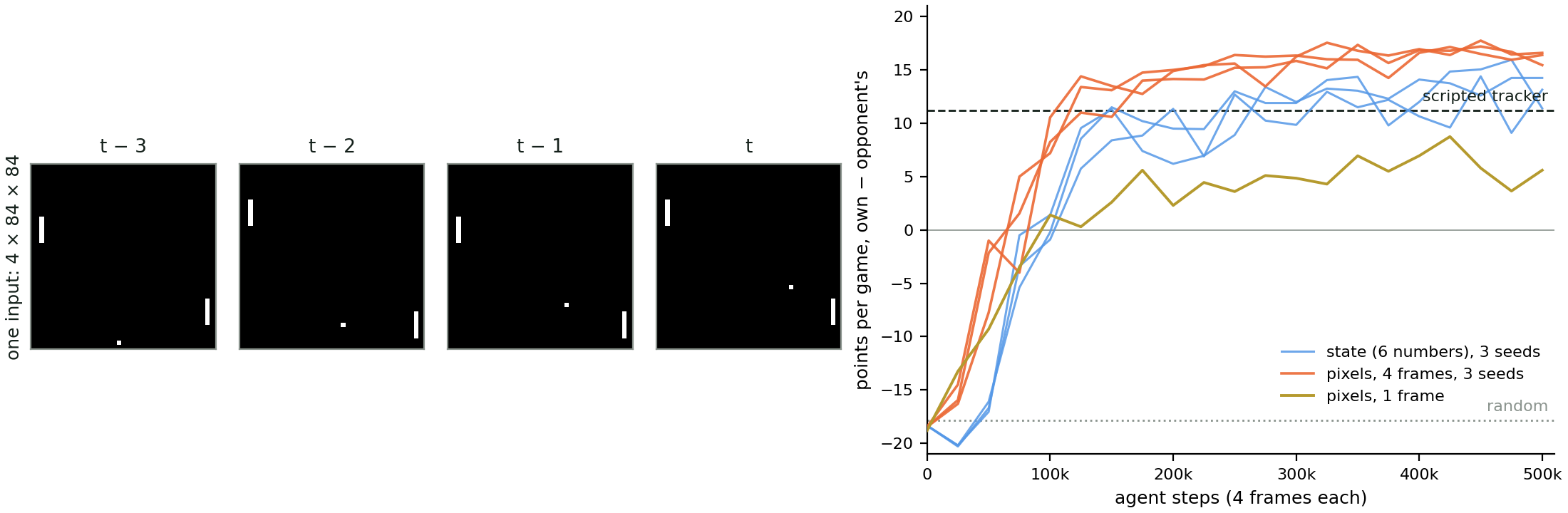
Every arm against the scripted opponent.

Table 13-1 is the mean points per game over twenty fresh games after training, with the standard error; the baselines over a hundred games (lake exe pong-env 100).

One frame cannot see velocity, and the row says by how much: \(+4.6\) against \(+15.5\), the gap between a paddle that reaches the ball and one that guesses. The state twin was meant to be the ceiling and is not: the pixel network sits above it on every seed (\(+15.47\) against \(+13.45\) on average) and at every opponent speed (1.0 / 1.5 / 2.0 pixels a frame: state \(+14.45\) / \(+13.45\) / \(+9.80\), pixels \(+17.75\) / \(+15.60\) / \(+14.45\)). The six numbers are all the pixels could carry, so the gap is in what each network learns from its input, and it is not dissected here. An update was 24 milliseconds, twenty of them the shim re-pushing 20 MB of parameters and Adam moments every step; with that state resident on the device (trainStepAdamF32DdpmR) it is 14.6, and a pixel run 27 minutes on one card.

13.2 Poker — Deep CFR against the exact best response

demos/MainDeepCfrLeduc.lean is Brown, Lerer, Gross and Sandholm’s loop (Deep CFR, ICML 2019, arXiv:1811.00164) on Leduc hold’em written in Lean (LeanMlir/Leduc.lean): a two-player, fixed-limit, one-card poker — \(r\) ranks in two suits, three for the classic jack–queen–king deck, an ante of one, two betting rounds with bets of two then four and at most two raises each, one public card between the rounds, a pair beats a higher rank — and the first game in this section with hidden information. The answer is therefore not a move but a mixed strategy: an equilibrium raises a jack it knows is losing about a fifth of the time, because a player who never bluffs can be read. Each iteration and player, one batched forward of the player’s advantage network over every information set gives the current strategy as a table (regret matching on the positive advantages), a thousand external-sampling traversals in C write instantaneous regrets to the player’s advantage reservoir and the opponent’s strategy to a strategy reservoir (reservoir sampling, a million rows each), and the advantage network is re-initialised and retrained from scratch on its reservoir, a thousand Adam steps at batch 512. After a hundred iterations the strategy network is trained on the strategy reservoir; Single Deep CFR (Steinberger 2019, arXiv:1901.07621) comes for free, the exact average of the hundred stored profiles weighted by iteration and by each profile’s own reach, no strategy network. The network is the Leduc papers’ three dense layers of 64 (Bestiary/DeepCFR.lean, 10.5k parameters, no BatchNorm), and the loss — a weighted squared error on the legal slots — goes through the squared-error block as a host-built target, tic-tac-toe’s move. Two things change relative to the three games around it:

• The instrument is the best response, and it is exact. Suits never matter in Leduc (there are no flushes), so the game is solved at rank level — \(6r + 30r^2\) information sets, 288 at \(r = 3\) against OpenSpiel’s 936 suit-aware ones, which fold onto them one-to-one — by vector-form CFR over the public tree with an \(r \times r\) matrix of private ranks at each node: the best response, exploitability (the best responder’s winnings per hand averaged over the two seats, OpenSpiel’s convention), head-to-head and CFR+ to a thousand iterations are 25 milliseconds at \(r = 3\) and under a second at \(r = 13\). Zero is Nash; CFR+ reaches \(2.4 \times 10^{-4}\). Before anything trains, the Lean game is checked against the C tree on every terminal history and both against OpenSpiel’s leduc_poker: every payoff on OpenSpiel’s own histories, and our tables scored by OpenSpiel’s exploitability to \(10^{-6}\) (scripts/demos/leduc_gate0_openspiel.py).

• The sampled table is the bracket, at the same budget. A table is enough at every \(r\) here, so the comparison is the Deep CFR paper’s own axis: exploitability against nodes touched, external-sampling MCCFR on a table against the network, at \(r = 3\), 6 and 13. The trainer’s own traversal with a lookup table in the network’s place must reproduce that curve before the network is trusted (mode=tabular), and does.

Figure 13-2 is one hand’s betting tree under the trained profile, the exploitability curves, and the bluff.

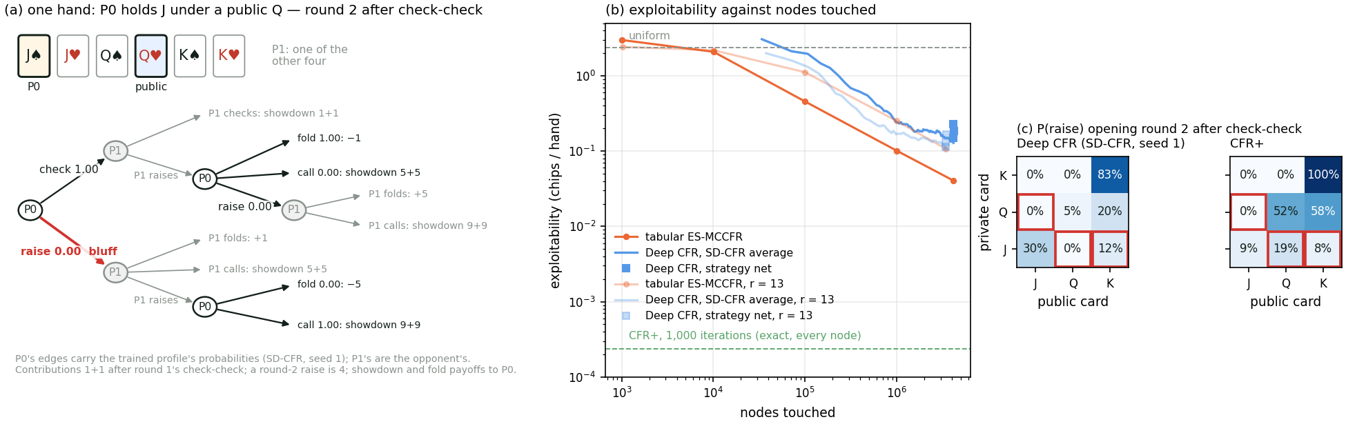
Every arm against the best response.

Exploitability in chips per hand (ante one; a thousandth of a chip is a milli-ante per game, the Leduc papers’ unit) and head-to-head against CFR+ averaged over the two seats. The scripted honest arm raises a pair or a king and folds a jack to a bet; the price-of-honesty arm is CFR+ with its worst-hand raises moved to call; the two Deep CFR rows and the sampled table are at the same 4.1M nodes, three seeds each. The last column of Table 13-2 is the bluff, the raise frequency opening round 2 with a jack under a queen.

Deep CFR’s exploitability falls from 1.4 at iteration 5 to 0.11–0.15 at a hundred and ends under the honest arm and under the equilibrium with its bluffs removed; at a hundred iterations it is where the Single Deep CFR paper’s Leduc curves are (150–200 milli-antes per game read from its Figure 1a, at 1,500 traversals an iteration to our thousand). It does not beat a sampled table at the same budget on the classic deck: the table is three times less exploitable at 4.1M nodes. The scale arm is where that turns. The same recipe at \(r = 6\) (1,116 sets) and \(r = 13\) (5,148): SD-CFR 0.112 / 0.123 / 0.113 against the table’s 0.053 / 0.066 / 0.058 at 3.6M nodes, then 0.099 / 0.120 / 0.106 against 0.113 / 0.107 / 0.102 at 3.4M — the table’s lead is \(3.1\times \), \(2.0\times \), \(1.0\times \), and at \(r = 13\) the network is the better head-to-head (\(-0.028\) against \(-0.035\) a hand). The table visits all but a set or two at these budgets, so the mechanism is not what it never saw; its estimate of each set is noisier as the sets multiply at a fixed budget, and the network’s error does not grow with them. The bluff column is the finding a reader can check on Figure 13-2: the trained profile that is 0.13 exploitable raises the losing jack under a queen 0% of the time where the equilibrium raises it 19.5% (18.6–19.5% over two solvers and three initialisations — the frequency is pinned at \(r = 3\), and is not at \(r = 13\), where the same cell ranges over tens of points), and it bluffs elsewhere instead, a jack under a king 12%. Honesty’s price is exact: moving the equilibrium’s worst-hand raises to call costs 0.186 of exploitability.

What this is not: a two-player, fixed-limit, one-card game, solved at rank level. The scale of the Deep CFR paper is heads-up flop and limit hold’em, where no exact best response exists to score against and the paper’s numbers are against abstractions and head-to-head; no-limit and multi-way poker (Pluribus) are another scale again, and exploitability is not computable there.

13.3 Tic-tac-toe — AlphaZero against the solved game

The demos/MainAlphaZeroTtt.lean trainer is Silver et al.’s self-play loop (AlphaGo Zero, 2017, Nature; AlphaZero, 2018, Science) on tic-tac-toe written in Lean (LeanMlir/TicTacToe.lean), \(n \times n\) with \(k\) in a row, \(n\) the one knob. Each iteration plays 256 games in lockstep: at every move a PUCT search of 25 (\(3 \times 3\)) or 100 (\(4 \times 4\)) simulations over the network’s priors and value, one batched forward over the games’ pending leaves per simulation, Dirichlet noise at the root, the move drawn from the visit counts; the visit distribution \(\pi \) and the outcome \(z\) are the targets, and the next iteration plays with the new network. The network is AlphaGo’s plain convolution + ReLU stack (Bestiary/AlphaGo.lean) at tic-tac-toe width, with the policy and value heads merged into one dense output of \(n^2 + 1\) slots: 78k parameters at \(3 \times 3\), 155k at \(4 \times 4\). Three things change relative to Pong’s DQN:

• The loss has two heads and the codegen has one. The paper’s \((z - v)^2 - \pi ^{\top } \log p\) goes through the squared-error block Pong’s Bellman target went through: the host runs the eval graph on the batch and writes \(y = \mathrm{out} - \tfrac {n_{\mathrm{out}}}{2}\, g\), with \(g = \mathrm{softmax}(p) - \pi \) on the \(n^2\) policy slots and \((\tanh v - z)(1 - \tanh ^2 v)\) on the value slot, so the block’s gradient is \(g / B\) exactly — the gradient of the batch-mean AlphaZero loss. Zero new codegen, the move the neural-quantum-state demo (§ 12.6) makes with its energy gradient.

• Not the bestiary’s tower. Bestiary/AlphaZero.lean’s convolution–BatchNorm–residual body is the wrong instrument here. BatchNorm’s batch statistics over nine binary cells are a liability, and with BatchNorm the eval forward the loss reads and the train step’s forward are different functions. Pong made the same choice for the same reason.

• The instrument is the solved game. A position is a base-3 number over the cells, so a memoised minimax fills one byte per index with the exact value and the optimal-move set of every reachable position — 5,478 at \(3 \times 3\), 9,722,011 at \(4 \times 4\). The network alone is scored by the argmax of its masked logits over every reachable decision position (4,520 and 9,062,619), its value head against the exact value, and its match play against a perfect player that draws uniformly from the optimal set. Nothing in the table is sampled but the games.

Five by five, four in a row.

No table exists there (\(3^{25}\) bytes), so the instrument becomes an exact solver — alpha-beta with a transposition table over symmetry-canonical positions — checked against the dense table on every reachable \(3 \times 3\) and \(4 \times 4\) position before it is trusted where no table exists. It establishes that \((5, 5, 4)\) is a draw, and something a reader can check on Figure 13-3: after X takes the centre, O’s only drawing replies are the four diagonal neighbours. Two things change in what the table can say: the sweep is a fixed sample of 20,000 random-play decision positions with at least six stones, exact per position but not exhaustive; and the perfect player draws its first move uniformly from the optimal set and plays the solver’s principal move from there.

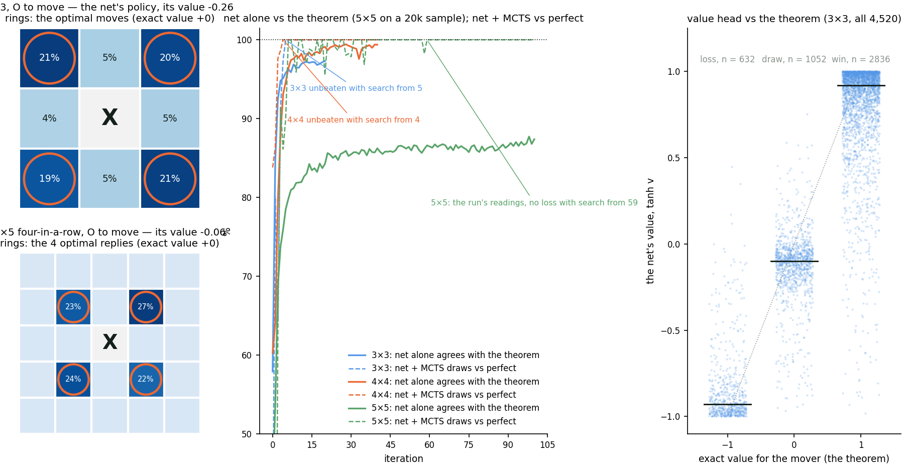
Every arm against the solved game.

Table 13-3 is the agreement of the arm’s move with the optimal set — over every decision position at \(3 \times 3\) and \(4 \times 4\), over the 20,000-position sample at \(5 \times 5\); the scripted players’ is their expected agreement — and W/D/L against the perfect player as X and as O: 1,000 games each way for the scripted rows (200 at \(5 \times 5\)), and for the network’s rows three independent evaluations of the saved network, 256 games each, pooled.

The Python implementation this loop follows (Nair, alpha-zero-general) was expected to take a day on the \(4 \times 4\) board. The untrained network’s sweep is the random player’s. Self-play visits 1.2% of the \(4 \times 4\) decision positions and the sweep scores all of them; the misses are mostly forced wins not taken, late in games a competent opponent never produces, and the search closes them — with 25 or 100 simulations the network is unbeaten from iteration 5 and 4, before the network alone is. The value head estimates self-play rather than the theorem (the right panel of Figure 13-3): the root ends X-favoured at \(3 \times 3\) because self-play under root noise is. At \(5 \times 5\) the same binary with n=5 k=4 runs a hundred iterations at 400 simulations in 64 minutes. As X the network never loses, alone or with search; as O it still does — 60 games in 768 alone, 23 with search — and its 87.4% on the random-play sample is 92.1% over the exhaustive opening, every position with at most three stones: it is best where the theory is. On this board the search is what closes the second player’s games, and it has not closed them yet.

13.4 Tic-tac-toe without the rules — MuZero against the solved game

The demos/MainMuZeroTtt.lean trainer is Schrittwieser et al.’s MuZero (2020, Nature) on the same instrument. AlphaZero is handed the rules: its search calls step. MuZero is not. Three plain convolution stacks — a representation \(h\) from the two stone planes to a \(32 \times n \times n\) latent, a dynamics \(g\) from a latent and a one-hot move plane to the next latent, and AlphaZero’s two-headed prediction \(f\) — plus a one-output reward network \(r\) on the latent a move reaches, 137k parameters at \(3 \times 3\) and 141k at \(4 \times 4\), are trained end to end on \(K = 5\) moves of stored games: the policy, value and reward targets at every unrolled step, the latent min–max normalised after every network as in the paper. The search is PUCT in the latent: a node is a path, one batched \(g\) over every game’s pending leaf per simulation, then one \(f\) and one \(r\); legal moves are masked at the root from the real rules and nowhere inside the tree. Win rate cannot tell this agent from AlphaZero — both are unbeaten — so the question the section asks is the one the solved game can answer exactly: did MuZero learn tic-tac-toe, or only its values? The literature predicts the second (Grimm et al. 2020’s value-equivalence principle; He, Moerland, de Vries and Oliehoek 2023 find MuZero’s model accurate on the policy it trained with and poor on others, measured against estimated returns). Here the answer is exact at every position, after every number of imagined moves, on lines the agent plays and lines it never would. Three things change relative to AlphaZero:

• One new codegen piece. The kit emits a train step — forward, backward and optimizer in one call — and an eval forward. MuZero’s loss reaches \(h\) and \(g\) through the unroll \(s_0 = h(o)\), \(s_{k+1} = g(s_k, a_k)\), so \(g\)’s backward has to hand a cotangent to the previous step and \(h\)’s receives the sum of everything downstream. MlirCodegen.generateVjp is the existing backward walk with the first layer’s input gradient — every convolution already emits one through conv2dHasVJP3, returned rather than dropped, with no optimizer tail; generateApplyAdam is the existing Adam update on its own. The trainer composes the gradient by hand, in reverse over the unroll, with the min–max’s VJP and the paper’s two scalings on the host. Gated before any game code: \(\theta - \partial \theta \) from the VJP module equals the SGD train step’s \(\theta '\) bit for bit on all 136,787 parameters of the four \(3 \times 3\) networks; the input cotangent agrees with central differences and with jax.vjp; the four composed gradients of the unrolled loss agree with jax.grad of the same loss written as one JAX function to \(7 \times 10^{-7}\) on the CPU compiler (on XLA’s CUDA path, \(2\)–\(7 \times 10^{-4}\): TF32 convolutions, the level every XLA-against-reference tie in this book sits at).

• A tree with no transpositions, gated against the one with them. AlphaZero’s search keys nodes by the true position’s index, so two move orders reaching one board share a node. A latent tree cannot: a node is a path. The gate that catches search bugs replaces \(g\) with the true dynamics — the latent of the real next position — and \(f \circ h\) with a trained AlphaZero network cut after its trunk, so both searches read the same two graphs: the position-keyed search’s first transposition needs seven simulations, so at \(2\) to \(6\) simulations every root visit distribution must agree exactly, and all 4,520 do; a planted bug that drops the edge reward passes at 2 and fails at 3–6 on 898–2,168 positions.

• The instrument scores the model, not only the player. From every reachable decision position (a fixed every-454th sample of the 9,062,619 at \(4 \times 4\)), a legal line of \(k = 0 \ldots 2K\) moves from three sources — the agent’s own policy, perfect play, uniform random legal moves — is played inside the model, and \(f(g^k(h(s)))\) is scored against the exact value and optimal set of the true position the line reaches; \(r\) against the true outcome of every move; and a closed-form ridge probe from the latent to the sixteen cell states, fit on \(h\) of real positions and refit on \(g\)’s own latents at each depth, says whether the board is still linearly decodable — the nearest thing to “knows the board”. Every number is exact per position; at \(3 \times 3\) every set is exhaustive.

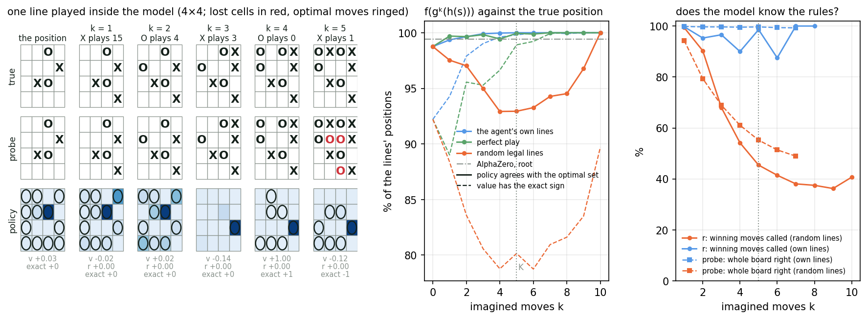
Every arm against the solved game.

Table 13-4 adds MuZero’s rows to Table 13-3’s protocol — agreement over every decision position, three independent 256-game evaluations of the saved network pooled against the perfect player — and two columns only a model can have: the policy’s agreement after \(K = 5\) imagined moves on the agent’s own lines and on random lines, and the share of winning moves \(r\) calls, over every legal move from every scored start. The networks are the recipe that passed at \(3 \times 3\) — 50-simulation self-play, 300 Adam steps an iteration, the raw mean \(Q\) — on fresh initialisations, 60 iterations at \(3 \times 3\) and 120 at \(4 \times 4\); at \(4 \times 4\) all three initialisations run end unbeaten both sides, alone and with 25 and 100 simulations, and the table’s is the one with the highest root agreement.

MuZero bootstraps slowly: AlphaZero’s \(4 \times 4\) network passes 93% root agreement by iteration 4, MuZero’s sits at 62–66% through iteration 40, 73% at 50, 92% at 60 and 98% by 100 — self-play stays decisive for a long time, so \(z\) teaches the values of weak play, and at \(4 \times 4\) sixty iterations is simply short. Doubling the steps an iteration brings the take-off to iteration 40 and the sweep to 99.1%, and costs one game in 256 alone as O. Self-play stood at 2.6% of the decision positions.

What the model learned.

The value-equivalent prediction — values, not the board — does not hold at one move and holds with depth. On the agent’s own lines the probe refit on \(g\)’s latents recovers 99.8% of whole \(4 \times 4\) boards after one imagined move and 99.7% after five; on random lines 94% after one and 55% after five, and a line of random moves is where Figure 13-4’s model loses the board. The reward network calls 99.5% of the winning moves at one move and 1.3% of the others; along random lines its recall falls to 45% by the fifth. The value’s sign holds on the agent’s own lines (92% at the root, 99.8% after five imagined moves, the surviving lines being endgames) and falls to 79–80% on random lines by the fourth — He et al.’s gap, against an exact value. Two move orders reaching one board land 2.0 apart in the latent, against 4.5 from \(h\) of that board and 5.2 between different boards: the model keeps the board in its own encoding, not \(h\)’s. The probe fit on \(h\) reads every held-out real position and 96–97% of the cells of \(g\)’s latents — at \(3 \times 3\) only 84%, and the weaker the network, the less of the board \(g\) keeps. What the search does with the model’s mistakes is the last line: at \(3 \times 3\) a third to a half of the positions where the search errs and the network alone does not carry a phantom win on the principal line — \(r\) calling a win the true board does not have — against 1–2% of other positions, and at the training budget extra simulations cost O games on two of three initialisations; at \(4 \times 4\) the search errs where the network alone does not at 3 starts in 19,961, one of them with a phantom win, and holds at 100 simulations on every initialisation.

13.5 The catalogue: the AlphaGo family and Deep CFR

The entries below are these loops at the scale that made them famous: the network is a residual tower, the game is Go or chess, and the target is still the model’s own later estimate.

Deep CFR (Bestiary/DeepCFR.lean)

Zero new primitives. Counterfactual regret minimisation with the two tables replaced by networks (Brown, Lerer, Gross and Sandholm 2019): an advantage network per player regresses the sampled counterfactual regrets of an information set and regret matching on its positive outputs is the current strategy; an average-strategy network regresses the strategies played, or, in Single Deep CFR (Steinberger 2019), the stored advantage networks are averaged exactly instead. The paper’s network is two branches — summed card embeddings through three dense layers, bet flags and sizes through two — concatenated into three more with skips where the widths agree and a normalisation of the last layer’s features, 98,948 parameters for heads-up flop hold’em; its Leduc experiments and ours use three dense layers of 64. The architecture is not the point and the paper says so; the loop is, and § 13.2 trains it.

def deepCfrLeducNet (r : Nat := 3) : NetSpec where
  name   := s!"Deep CFR Leduc r{r}"
  imageH := 1
  imageW := 1
  layers := [
    -- 2r + 24 features: one-hot cards with rank scalars, pair and
    -- above-public flags, the betting history, the round, the pot.
    .dense (2 * r + 24) 64 .relu,
    .dense 64 64 .relu,
    .dense 64 64 .relu,
    .dense 64 3 .identity          -- fold, call, raise
  ]

AlphaGo (Bestiary/AlphaGo.lean)

Zero new primitives. The original 2016 Lee Sedol system (Silver et al. 2016, Nature). Three separate networks: a 13-layer conv policy network (\(\sim \)3.9M) trained first on 30M human games then fine-tuned via self-play, a 13-layer conv + FC-head value network (\(\sim \)4M), and a shallow linear rollout policy used inside MCTS for fast tree playouts. Input is 48 hand-crafted Go feature planes (liberties, ladder patterns, 3\(\times \)3 stone arrangements, etc.). AlphaGo Zero (next entry) throws all of this out — raw board only, one two-headed net, self-play only — and plays better (5185 Elo vs 3140). The one-sentence lesson is written into every follow-up paper: features the network can learn on its own, it will.

def alphaGoPolicyNet : NetSpec where
  name   := "AlphaGo policy network"
  imageH := 19
  imageW := 19
  layers := [
    -- 13 conv layers: one 5×5 stem + eleven 3×3 at 192 channels.
    -- Plain conv+ReLU, no BatchNorm: 2016 AlphaGo predates both BN and
    -- residual blocks in this lineage (AlphaGo Zero added them).
    .conv2d 48 192 5 .same .relu,                 -- 48 hand-crafted planes in
    .conv2d 192 192 3 .same .relu, .conv2d 192 192 3 .same .relu,
    .conv2d 192 192 3 .same .relu, .conv2d 192 192 3 .same .relu,
    .conv2d 192 192 3 .same .relu, .conv2d 192 192 3 .same .relu,
    .conv2d 192 192 3 .same .relu, .conv2d 192 192 3 .same .relu,
    .conv2d 192 192 3 .same .relu, .conv2d 192 192 3 .same .relu,
    .conv2d 192 192 3 .same .relu,
    -- 1×1 conv to per-position move logit (reshape + pass scalar downstream)
    .conv2d 192 1 1 .same .identity
  ]

AlphaZero (Bestiary/AlphaZero.lean)

Zero new primitives — convBn + residualBlock + dense. Two-headed (policy + value) network (Silver et al. 2018, arXiv:1712.01815), expressed as two separate NetSpec values sharing the body in prose. Variants: AlphaGo Zero (Go; Silver et al. 2017, Nature), AlphaZero chess, tiny fixture.

def alphaGoZeroPolicy : NetSpec where
  name   := "AlphaGo Zero (policy head)"
  imageH := 19
  imageW := 19
  layers := [
    .convBn 17 256 3 1 .same,                     -- 17 raw-history planes → 256
    .residualBlock 256 256 19 1,                  -- 19 residual blocks (shared body)
    .convBn 256 2 1 1 .same,                      -- policy head: conv→BN→ReLU (2 filters)
    .flatten,
    .dense (2 * 19 * 19) 362 .identity            -- 361 board moves + pass
  ]

The value head shares the first two layers (body) and diverges at the head — one filter, two-layer MLP down to a single scalar (tanh is applied downstream; Activation doesn’t include it):

def alphaGoZeroValue : NetSpec where
  name   := "AlphaGo Zero (value head)"
  imageH := 19
  imageW := 19
  layers := [
    .convBn 17 256 3 1 .same,                     -- shared body
    .residualBlock 256 256 19 1,                  -- shared body
    .convBn 256 1 1 1 .same,                      -- value head: conv→BN→ReLU (1 filter)
    .flatten,
    .dense (1 * 19 * 19) 256 .relu,
    .dense 256 1 .identity                        -- → scalar (tanh applied downstream)
  ]

The chess variant keeps the 19-block tower on 119 input planes over an \(8 \times 8\) board, and its policy head is convolutional as in Silver et al. 2018: a convolution to 73 move planes, flattened into the 4672 logits, with no dense layer. The tiny fixture is 17 planes, 3 blocks, a \(9 \times 9\) board.

MuZero (Bestiary/MuZero.lean)

Zero new primitives — three ResNet-style networks (representation, dynamics, prediction) reusing convBn + residualBlock + dense. The architectural novelty is the three-network factoring, not any single layer type (Schrittwieser et al. 2020, arXiv:1911.08265). Five NetSpec values per variant (rep, dyn body, dyn reward head, pred policy, pred value). Variants: Go, Atari (representation only), tiny.

def muZeroGoRepresentation : NetSpec where
  name   := "MuZero Go — representation h"
  imageH := 19
  imageW := 19
  layers := [
    .convBn 17 256 3 1 .same,                     -- observation → hidden
    .residualBlock 256 256 16 1                   -- 16 ResBlocks (AlphaZero-shaped body)
  ]

The dynamics network \(g\) takes the hidden state plus a one-channel action plane and predicts the next hidden state. A separate reward head branches off the same trunk and emits a scalar:

def muZeroGoDynamics : NetSpec where
  name   := "MuZero Go — dynamics g (next-state path)"
  imageH := 19
  imageW := 19
  layers := [
    .convBn 257 256 3 1 .same,                    -- 256 hidden + 1 action plane
    .residualBlock 256 256 16 1                   -- → next hidden (256, 19, 19)
  ]

def muZeroGoDynamicsReward : NetSpec where
  name   := "MuZero Go — dynamics g (reward head)"
  imageH := 19
  imageW := 19
  layers := [
    .convBn 256 1 1 1 .same,                      -- 1×1 conv→BN→ReLU to 1 channel
    .flatten,
    .dense (1 * 19 * 19) 128 .relu,
    .dense 128 1 .identity                        -- scalar reward
  ]

The prediction network \(f\) is a small two-headed body — same shape as AlphaZero’s policy/value heads, with two fewer ResBlocks because the trunk has already done most of the work in \(h\):

def muZeroGoPredictionPolicy : NetSpec where
  name   := "MuZero Go — prediction f (policy head)"
  imageH := 19
  imageW := 19
  layers := [
    .residualBlock 256 256 2 1,                   -- small head body
    .convBn 256 2 1 1 .same,                      -- policy head: conv→BN→ReLU (2 filters)
    .flatten,
    .dense (2 * 19 * 19) 362 .identity            -- 361 moves + pass
  ]

def muZeroGoPredictionValue : NetSpec where
  name   := "MuZero Go — prediction f (value head)"
  imageH := 19
  imageW := 19
  layers := [
    .residualBlock 256 256 2 1,
    .convBn 256 1 1 1 .same,                      -- value head: conv→BN→ReLU (1 filter)
    .flatten,
    .dense (1 * 19 * 19) 256 .relu,
    .dense 256 1 .identity                        -- scalar value
  ]