6 MobileNetV2

A standard conv does two jobs at once

A standard 3\(\times \)3 convolution from \(C_\text {in}\) channels to \(C_\text {out}\) channels computes, for every output cell:

That sum is doing two things. The \(k_h, k_w\) part is spatial mixing: it combines a pixel with its neighbors. The \(c_\text {in}\) part is cross-channel mixing: it combines the \(C_\text {in}\) channels into each of \(C_\text {out}\) new channels. Both happen inside the same kernel and at the same cost \(C_\text {in} \times C_\text {out} \times k^2\) weights per layer.

Howard et al. 2017 (MobileNetV1, arXiv:1704.04861) and Sandler et al. 2018 (MobileNetV2, arXiv:1801.04381) asked: what if we factored those two responsibilities and only paid the full cost of one of them? The spatial mixing is locally information-rich and benefits from a real \(3 \times 3\) neighborhood. The channel mixing can be approximated by a much cheaper operation. If we separate them, we get parameter efficiency without losing much expressive power.

6.1 Run it first

Before the factorization, train the factorized network. Four commands, and about thirty-five minutes of GPU time:

lake exe cache get                            # Mathlib oleans, ~30 s
./scripts/datasets/download_imagenette.sh     # 330 MB dl, 2.4 GB unpacked
lake build mobilenetv2-verified-adam
./.lake/build/bin/mobilenetv2-verified-adam data

On one RTX 4060 Ti (CUDA 12.9), from runs/2026-08-12-mnv2-imagenette-xla-cuda/. XLA’s startup banner is removed, the network description line is wrapped, and the middle of the run is elided:

[pjrt_ffi] XLA backend: PJRT 0.112, 1 device(s)
[pjrt_ffi] compiled verified_mlir/mobilenetv2_adam_train_step.mlir
             (@mobilenetv2_adam_train_step, 581 outputs, 1 replica) in 8101 ms
[pjrt_ffi] compiled verified_mlir/mobilenetv2_fwd.mlir
             (@mobilenetv2_fwd, 1 outputs, 1 replica) in 665 ms
[pjrt_ffi] compiled verified_mlir/mobilenetv2_fwd_eval.mlir
             (@mobilenetv2_fwd_eval, 1 outputs, 1 replica) in 250 ms
MobileNetV2 on Imagenette 224² (stem-s2 → 17 inverted-residual blocks,
  full-paper [t,c,n,s] config, stride-2 depthwise downsamples 224→7 →
  head conv-BN-relu6 → GAP → dense)
  via the VERIFIED renderer → XLA/PJRT → GPU
  train 9469, val 3925; bs 32, MobileNetV2 adam
    (cosine+warmup 3ep, baseLR 0.001000), He init
  running-stats BN: 52 layers, 34112 stat floats → eval via @mobilenetv2_fwd_eval
Epoch 1/80: loss=2.121050 lr=0.000333
  epoch 1: val_acc = 947/3925 = 24.127389%  top5 = 2392/3925 = 60.942675%
Epoch 2/80: loss=1.784318 lr=0.000667
  epoch 2: val_acc = 680/3925 = 17.324841%  top5 = 2357/3925 = 60.050955%
Epoch 3/80: loss=1.590689 lr=0.001000
  epoch 3: val_acc = 1596/3925 = 40.662420%  top5 = 3423/3925 = 87.210191%
Epoch 4/80: loss=1.446373 lr=0.001000
  epoch 4: val_acc = 1851/3925 = 47.159236%  top5 = 3428/3925 = 87.337580%
Epoch 79/80: loss=0.517682 lr=0.000000
  epoch 79: val_acc = 3506/3925 = 89.324841%  top5 = 3874/3925 = 98.700637%
Epoch 80/80: loss=0.517213 lr=0.000000
  epoch 80: val_acc = 3503/3925 = 89.248408%  top5 = 3873/3925 = 98.675159%
done (trained MobileNetV2 adam + cosine/warmup via packed threading).

Eighty epochs at about 26 seconds each, thirty-five minutes in total, and 89.25% top-1 with 98.68% top-5 on Imagenette’s 3,925-image validation split. The best epoch reached \(89.32\% \). Set that against Chapter 5, which ran the same data, the same recipe and the same number of epochs through a network with \(9.5\times \) the parameters and averages \(89.99 \pm 0.32\) top-1 over five seeds (runs/2026-09-12-r34-ablation-fp32-seeds/). MobileNetV2 gives up three quarters of a point of top-1 — less than one run’s own \(\pm 0.97\) interval — picks up a fifth of a point of top-5, and does it in thirty-five minutes against forty-seven.

Epoch 2 is worth a glance before moving on. Validation accuracy falls, from \(24.1\% \) to \(17.3\% \), while the training loss drops normally. The learning rate is still warming up and the BatchNorm running statistics are averaging over weights that are moving fast, so the evaluation forward — @mobilenetv2_fwd_eval, the third artifact every BatchNorm net compiles, fed by the running-stats BN line above it — is using statistics that no longer describe the thing being evaluated. It corrects itself by epoch 3 and never recurs.

One scope note, because this is the chapter where the distinction starts to bite. The theorem that folds this run’s backward into a single statement about the whole network, Theorem 82, is pointwise: it holds at a given input, and it carries one side condition per activation site, thirty-five per example, saying that the value entering relu6 is neither \(0\) nor \(6\). relu6 has two corners, the network is not differentiable at them, and a statement quantified over all inputs would be false. Chapter 7 folds EfficientNet-B0 over all inputs because swish is smooth everywhere; what moved here was the depth, from two blocks to seventeen, not the pointwise-to-global axis.

Depthwise: one kernel per channel, no cross-channel sum

A depthwise convolution does the spatial half on its own, per channel. Each output channel comes from one input channel, with its own \(k \times k\) kernel:

Only one summation level (over the kernel positions), not two. No mixing between channels at all. Channel \(c\) of the output only ever looks at channel \(c\) of the input. The weight tensor is shape \([C, k, k]\) instead of \([C_\text {out}, C_\text {in}, k, k]\):

For a typical \(C_\text {in} = C_\text {out} = 64\) layer, that is 576 weights against 36,864, a 64\(\times \) reduction. The Jacobian from Chapter 3 simplifies in step: one fewer \(\Sigma \) level means the depthwise input-VJP is a slightly simpler reversed-kernel convolution, the weight VJP is a slightly simpler transpose-trick, and the bias VJP is the same per-channel sum. Theorems 79 through 81 prove the depthwise VJPs.

The depthwise-separable sandwich

A depthwise conv alone never lets channels see each other. That is a problem, because the whole point of stacking convolutions is to build hierarchical features that combine information across channels. The fix is to follow each depthwise with a pointwise \(1 \times 1\) convolution, which is purely cross-channel mixing (no spatial structure, since each output pixel is a learned linear combination of the same input pixel’s channels). That two-step combination,

is called a depthwise-separable convolution, and it is what replaces the standard \(3 \times 3\) conv in MobileNet and everywhere downstream. A standard \(3 \times 3\) over 64\(\to \)64 costs 36,864 weights. The separable version costs 576 (depthwise) plus 4,096 (pointwise), for 4,672. Eight times fewer.

Inverted residual: depthwise at the wide point

MobileNetV2 wraps the separable block in one more idea. ResNet’s bottleneck block is wide \(\to \) narrow \(\to \) wide (project down for the expensive spatial conv, project back up for the residual). MobileNetV2 flips it: narrow \(\to \) wide \(\to \) narrow, with the depthwise spatial conv at the wide expansion. The intuition is that depthwise is so cheap that you can afford to make it wider. The narrow bottleneck channels carry the actual information across the residual.

Concretely, an inverted-residual block with input channels \(C_\text {in}\), output channels \(C_\text {out}\), and expansion ratio \(t\):

1. \(1 \times 1\) conv \(C_\text {in} \to t \cdot C_\text {in}\) (the expand)

2. \(3 \times 3\) depthwise at \(t \cdot C_\text {in}\) channels (the spatial mix at the wide point)

3. \(1 \times 1\) conv \(t \cdot C_\text {in} \to C_\text {out}\) (the project, narrowing back down)

4. Residual skip when \(C_\text {in} = C_\text {out}\) and stride equals 1

This is the .invertedResidualNB ic mid oc stride primitive in the spec, one layer constructor that emits all three convs, the BN and relu6 between them, and the conditional residual add. It takes the expanded width mid directly rather than the ratio \(t\), so a block is written the way it is shaped rather than the way it is parameterized, and the NB suffix says the three convs carry no bias, since the BatchNorm immediately after each one subsumes it. The VJP for the whole block composes the depthwise VJP from this chapter with the conv2d VJP (Theorem 35), the BN VJP (Theorem 50) and the residual’s additive fan-in (Theorem 64). Once again there is no new math beyond the foundation rules, only the depthwise primitive plus composition.

Stacking the blocks

MobileNetV2 stacks 17 inverted-residual blocks across seven stages (at depths 1, 2, 3, 4, 3, 3, 1) with widths progressing from 16 to 320 channels, then a final \(1 \times 1\) to 1280 channels, global average pool, and a 1280-to-10 dense head. That is the same stem-stages-head template as ResNet-34. Total: 2.24M parameters, 9.5\(\times \) fewer than ResNet-34, at a modest accuracy cost (\(89.25\% \) against ResNet-34’s \(89.99\% \) on Imagenette, both measured in this book). For mobile and embedded deployment that trade is the whole reason MobileNet exists.

6.2 The theorems

Figure 6-1 is the dependency graph of this section.

The ladder of Chapter 5, twice: MobileNetV2 and MobileNetV4-Conv-M take each of the six rungs in turn.

6.3 Example: MobileNet V2 on Imagenette

The architecture

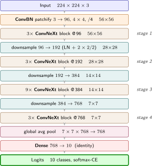
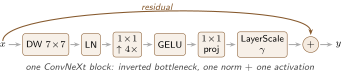
The same vertical column as ResNet-34, now built from inverted-residual blocks: a \(3 \times 3\) stride-2 stem, seven stages of .invertedResidualNB blocks (17 in all, widths \(16\) to \(320\), expansion \(t{=}6\) except the first), a \(1 \times 1\) lift to 1280 channels, global average pool, and a dense head. There are no max-pools, since every downsample is folded into a strided block. Figure 6-2 is the network, and its inset shows one inverted-residual block: the cheap depthwise spatial mix happens at the wide point.

The verified trainer

§5-2 is the pattern and this is the first chapter to reuse it, so read the two together. Everything that carries weight there carries the same weight here, and only the layers list and the bnChannels that follows from it are new:

import LeanMlir.Verified.NetsCore
import LeanMlir.Verified.Train

-- 1. The network. `slug` names the committed render, `runningBN`
--    turns on the running-statistics threading (the 52 slots are
--    read off `layers`), `NB` means the convs carry no bias.
def mobilenetv2Verified : VerifiedNetSpec where
  name     := "MobileNetV2"
  slug     := "mobilenetv2"
  inC      := 3
  imageH   := 224
  imageW   := 224
  data     := .imagenette
  layers   := [
    .convBnNB 3 32 3 2,                   -- stem (no conv bias)   224->112
    .invertedResidualNB 32  32  16 1,     -- stage 1, t=1
    .invertedResidualNB 16  96  24 2, .invertedResidualNB 24 144  24 1,  -- 112->56
    .invertedResidualNB 24 144  32 2, .invertedResidualNB 32 192  32 1,
    .invertedResidualNB 32 192  32 1,
    .invertedResidualNB 32 192  64 2, .invertedResidualNB 64 384  64 1,
    .invertedResidualNB 64 384  64 1, .invertedResidualNB 64 384  64 1,
    .invertedResidualNB 64 384  96 1, .invertedResidualNB 96 576  96 1,
    .invertedResidualNB 96 576  96 1,
    .invertedResidualNB 96 576 160 2, .invertedResidualNB 160 960 160 1,
    .invertedResidualNB 160 960 160 1,
    .invertedResidualNB 160 960 320 1,    -- stage 7 @7
    .convBnNB 320 1280 1 1,         -- head (no conv bias), 1x1 to 1280
    .globalAvgPool,
    .dense 1280 10 ]
  runningBN  := true

-- 2. The schedule. Identical to ResNet-34's, deliberately.
def mobilenetv2AdamConfig : VerifiedConfig where
  epochs    := 80
  batchSize := 32

-- 3. The entry point: AdamW, cosine with a 3-epoch warmup, baseLR 1e-3.
--    LEAN_MLIR_VARIANT=rms selects the RMSProp render and its own rate.
def runMobilenetV2Adam (argv : List String) : IO Unit := do
  let variant := (← IO.getEnv "LEAN_MLIR_VARIANT").getD "adam"
  let sched := mnv2RmsSchedule
  let rms := variant.startsWith "rms"
  let bs := mobilenetv2AdamConfig.batchSize
  let baseLR := match (← IO.getEnv "LEAN_MLIR_BASE_LR_U").bind (·.toNat?) with
    | some u => u.toFloat * 1e-6
    | none   => if rms then sched.lr * bs.toFloat / 256.0 else 0.001
  mobilenetv2Verified.toNet.trainAdamSched mobilenetv2AdamConfig
    (argv.head?.getD "data") baseLR 0.9 0.999 3 variant
    (if rms then sched.decayRate else 0.0) sched.decayEpochs
def main (argv : List String) : IO Unit := runMobilenetV2Adam argv

Every block is its own line, with no repeat count, because one constructor is one block. The constructor .invertedResidualNB ic mid oc stride takes the expanded width mid rather than a ratio \(t\), so the widths read straight off the paper’s table and the stage boundaries are visible as the places where stride is 2. Internally each block is a \(1 \times 1\) conv to mid channels, a \(3 \times 3\) depthwise at that width, a \(1 \times 1\) project to oc, and a residual skip when ic == oc and stride == 1. Its VJP is Theorem 79 for the depthwise conv composed with the dense, BN and biPath theorems already proved.

The BatchNorm list has 52 entries, not the 53 a per-block count gives. Every inverted-residual block normalizes after each of its three convs, which would be \(17 \times 3 + 2\) for the stem and head, or 53. The first block has expansion \(t{=}1\), so it has no expand conv at all and contributes two entries rather than three, and the real count is 52. That is the kind of detail bnChannels exists to get right: the running-stat region is positional, and an off-by-one there misaligns every frozen statistic downstream of it at evaluation time.

The toSpecs arm carries the same count. .invertedResidualNB is one more entry on Chapter 1’s toSpecs, and the \(t{=}1\) carve-out above is not prose — it is the conditional:

  | invertedResidualNB ic mid oc _ =>          -- Ch. 6
    (if mid != ic then #[(#[mid,ic,1,1],0),(#[mid],1),(#[mid],2)] else #[])
    ++ #[(#[mid,1,3,3],0),(#[mid],1),(#[mid],2),      -- depthwise 3x3 + BN
         (#[oc,mid,1,1],0),(#[oc],1),(#[oc],2)]       -- project 1x1 + BN

mid != ic is exactly “\(t \neq 1\)”. When it holds the block contributes nine tensors and three BatchNorms; when it fails the expand conv is not emitted at all and the block contributes six and two. Sixteen blocks at three plus one at two, plus the stem and the head, is the 52. The depthwise kernel is [mid,1,3,3] — one filter per channel, which is the whole of Theorem 79’s subject written as a shape.

The recipe is ResNet-34’s, unchanged. Eighty epochs at batch 32, AdamW at \(10^{-3}\), cosine with a three-epoch warmup, label smoothing \(0.1\), the same augmentation. That is on purpose. Holding the recipe fixed is what makes the accuracy in §6.1 a comparison between two architectures rather than between two training setups, and it is the same move Chapter 4 used to compare optimizers against one proven gradient. MobileNetV2’s own optimizer is RMSProp, which §6.5 comes back to, and it is rendered at this shape too: LEAN_MLIR_VARIANT=rms loads mobilenetv2_rms_train_step.mlir instead.

Results

§6.1 has the run: 80 epochs at about 26 seconds each on one RTX 4060 Ti, finishing at 89.25% top-1 and 98.68% top-5 on Imagenette’s 3,925-image validation split. Against Chapter 5’s ResNet-34 at \(89.99 \pm 0.32\) (runs/2026-09-12-r34-ablation-fp32-seeds/) on the same data and the same recipe, that is 0.74 points of top-1 for 9.5\(\times \) fewer parameters (2.24M against 21.3M). That is the depthwise-separable trade, and on this evidence it is a better one than the architecture’s reputation suggests. From the log:

• 2.24M parameters, and 1.07 MB of MLIR (1 070 905 chars) for the AdamW training step. ResNet-34 emitted 754 KB with \(9.5\times \) the parameters, so the smaller network renders the larger program. Emission is per-op, and the separable block trades one convolution for three, each with its own BatchNorm. Parameter count went down and operation count went up, and the text follows the second.

• Per-step time is about 90 ms at batch 32, against ResNet-34’s 120 ms at the same batch, the same 295 steps to the epoch and the same resident parameters, so the whole run takes thirty-five minutes rather than forty-seven. That is a real \(1.3\times \), and it is far short of what the parameter count promises: \(9.5\times \) fewer weights buys \(1.3\times \) the throughput, not \(9.5\times \). Depthwise convolution is memory-bound. It does nine multiply-accumulates per output element where the standard \(3 \times 3\) it replaces does \(9 C_\text {in}\), so the kernel spends its time moving activations rather than multiplying them, and arithmetic was never the whole bottleneck. §6.5 sees the same sub-proportional scaling at ImageNet.

• The net renders as three artifacts. The train step is accompanied by mobilenetv2_fwd (152 793 chars) and mobilenetv2_fwd_eval (120 698 chars), the second existing only because BatchNorm evaluates differently than it trains. It is the concrete cost of the bnChannels line in the spec above.

• 52 BN layers, up from ResNet-34’s 36, for the same reason the MLIR is bigger: more internal convolutions means more BN-after-conv pairs. Each one still proves its VJP via Theorem 50.

• Final loss plateaus near 0.50 again. The label-smoothing floor at \(\varepsilon = 0.1\) over ten classes is \(0.500\), the entropy of the \(0.91 / 0.01\) target, and this run’s final \(0.517\) sits just above it: converged rather than stalled.

6.4 MLIR: Depthwise Convolution

What is already proven. A depthwise convolution applies one \(k\times k\) kernel per channel with no cross-channel sum, so its reverse-mode derivative (Theorem 79, depthwiseHasVJP3) is a reversed-kernel convolution minus the channel transpose the full-conv VJP (Theorem 35) needs: with no \(\sum _{c_\text {in}}\) to take the adjoint of, there is no in/out channel axis to swap. The inverted-residual block composes this with the pointwise convs, BatchNorm, and relu6, and mobilenetv2ForwardBFullHasVJPAt chains the whole network through vjpCompAt.

The gap and how we close it. The emitted graph is denoted and shown equal to depthwiseHasVJP3’s backward. Here is the depthwise input gradient in verified_mlir/mobilenetv2_adam_train_step.mlir, at the last inverted-residual block (960 channels at \(7\times 7\), \(3\times 3\) kernels, batch 32; SSA names the artifact’s, lines wrapped):

%v1729 = stablehlo.reverse %b17dW, dims = [2, 3] : tensor<960x1x3x3xf32>
%v1730 = stablehlo.convolution(%v1728, %v1729)
      dim_numbers = [b, f, 0, 1]x[o, i, 0, 1]->[b, f, 0, 1],
      window = {stride = [1, 1], pad = [[1, 1], [1, 1]],
      lhs_dilate = [1, 1], rhs_dilate = [1, 1]}
      {batch_group_count = 1 : i64, feature_group_count = 960 : i64}
      : (tensor<32x960x7x7xf32>, tensor<960x1x3x3xf32>)
      -> tensor<32x960x7x7xf32>

Read it against Chapter 3’s convolution backward. That one swapped the kernel’s in- and out-channel axes with a transpose before reversing; this one has no transpose. The depthwise kernel is stored as \([c, 1, k, k]\), one \(3\times 3\) filter per channel with a singleton input-channel axis, so the reverse at %v1729 flips its two spatial axes and nothing else, and feature_group_count = 960, equal to the channel count, tells the convolution at %v1730 to run each channel of the cotangent %v1728 through its own filter with no mixing. That single attribute is the depthwise structure. The leaf theorem is depthwiseBackBatched_faithful: this node denotes the backward of the batched depthwise convolution, which, the operator being linear, is the per-example backward applied row by row, and depthwiseFlatBack_eq_vjp_backward is that per-example backward’s identification with depthwiseHasVJP3, for odd kernels. Theorem 86 threads it through the seventeen blocks.

Caveats.

• The depthwise convolution bridge holds at every input, because the op is linear; its one hypothesis is an odd kernel (depthwiseFlatBack_eq_vjp_backward), and MobileNetV2’s are all \(3\times 3\).

• relu6 is a smooth-point bridge. MobileNetV2’s clamp to \([0,6]\) has no derivative where a pre-activation sits exactly at \(0\) or \(6\), and the bridge is stated only off that set, null for generic weights.

• Shape. The listing is one block of the trained net; the theorem is stated at every channel count and odd kernel size.

6.5 ImageNet recipe

The Imagenette run above trained on \(\sim \)9.5K images. The same backbone scales to full 1000-class ImageNet exactly the way ResNet-34 did in Chapter 5: the inverted-residual stack is unchanged, only the head widens to 1000 and the dataset and schedule grow. As there, the recipe runs on both paths — the reference first, then the verified path, then the two side by side.

The reference (JAX)

The reference trainer is jax/MainMobilenetV2Imagenet.lean; its spec, and its recipe, as the run below trained it:

-- Same inverted-residual backbone, 1000 classes instead of 10.
def mobilenetV2Imagenet : NetSpec where
  name   := "MobileNetV2 (ImageNet, bf16)"
  imageH := 224
  imageW := 224
  convBnAct := .relu6               -- ReLU6 throughout, stem and 1x1 head included
  layers := [
    .convBn 3 32 3 2 .same,
    .invertedResidual  32  16 1 1 1,
    .invertedResidual  16  24 6 2 2,
    .invertedResidual  24  32 6 2 3,
    .invertedResidual  32  64 6 2 4,
    .invertedResidual  64  96 6 1 3,
    .invertedResidual  96 160 6 2 3,
    .invertedResidual 160 320 6 1 1,
    .convBn 320 1280 1 1 .same,
    .globalAvgPool,
    .dense 1280 1000 .identity      -- 1000-class head
  ]

-- TF-slim's README command, row for row; the table below names each value's source.
def mobilenetV2ImagenetConfig : TrainConfig where
  learningRate   := 0.12      -- 0.045 per 96 images, scaled to 256
  batchSize      := 256
  epochs         := 90        -- the validation tier; `full` is ~420
  optimizer      := .rmsprop  -- slim's default optimizer
  momentum       := 0.9       -- rmsprop_momentum
  rmspropDecay   := 0.9       -- rmsprop_decay
  rmspropEps     := 1.0       -- opt_epsilon (NOT 1e-8)
  rmspropTf      := true      -- TF1 ApplyRMSProp: the rate inside the momentum term
  weightDecay    := 4e-5      -- coupled, the regularization loss
  wdExcludeNormBias := true   -- decay on conv2d kernels only: no BN γ/β, no biases
  wdExcludeDepthwise := true  -- …and not on the depthwise kernels
  initTruncNormal := 0.09     -- truncated normal on every kernel and the logits
  cosineDecay      := false   -- exponential_decay instead
  expLRDecayRate   := 0.98    -- learning_rate_decay_factor
  expLRDecayEpochs := 2.5     -- num_epochs_per_decay, in epochs of data
  expLRStaircase   := true    -- staircase=True, counted from step 0
  dropout          := 0.2     -- dropout_keep_prob 0.8
  warmupEpochs   := 0         -- warmup_epochs unset
  augment        := true      -- inception_preprocessing: distorted crop + flip
  cropAreaMin    := 0.05      -- area_range (0.05, 1.0)
  cropMaxAttempts := 100      -- …then the whole image
  cropAspectLo   := 0.75      -- aspect_ratio_range (0.75, 1.33)
  cropAspectHi   := 1.33
  trainResize    := .bilinear -- resize_images, fast_mode
  resizeAntialias := false    -- resize_images: no antialias
  resizeLegacyTf1 := true     -- TF 1's resize_bilinear kernel, train and eval
  colorDistortSlim := true    -- distort_color fast_mode: brightness, then saturation
  inputScalePm1  := true      -- (x − 0.5) × 2
  evalCropTf     := true      -- preprocess_for_eval: crop first, then resize
  evalCropSlim   := true      -- central_crop(0.875) of both sides, then resize to 224
  useAutoAugment := false     -- none in slim's pipeline
  labelSmoothing := 0.1       -- --label_smoothing=0.1
  useEMA         := true      -- --moving_average_decay=0.9999
  emaDecay       := 0.9999
  emaWarmup      := true      -- ExponentialMovingAverage with num_updates
  evalF32        := true      -- the reference number from an f32 forward
  bf16           := true
  bf16Conv       := true      -- reaches the inverted-residual blocks
  f32StemHead    := true      -- classifier head in fp32, as every verified render
  runningBN      := true      -- paper-faithful eval: running BN stats
  bnMomentum     := 0.997     -- bn_decay 0.997 (PyTorch momentum 0.003)
  bnEps          := 1e-3      -- slim.batch_norm's ε

/-- The run: the README's "about 700K steps" on 8 clones of 96, which is
    700,000 × 768 / 1,281,167 ≈ 420 epochs of data. Selected with the `full`
    recipe arg; writes a separate `_full.py` so a quick validation subrun and
    the multi-day run never clobber each other. -/
def mobilenetV2ImagenetConfigFull : TrainConfig :=
  { mobilenetV2ImagenetConfig with epochs := 420 }

Table 6-1 is where each value of the config comes from.

The run below is mobilenetV2ImagenetConfigFull, launched by scripts/jobs/mnv2-full-jax-4gpu.conf. The recipe is not the paper’s sentence but TF-slim’s own reproduction command (research/slim/nets/mobilenet/README.md), read with the sources it runs: \(0.045\) per \(96\) images, so \(0.12\) at \(256\), stepped \(\times 0.98\) every \(2.5\) epochs of data as a staircase from step \(0\) with no warmup; TF 1’s RMSProp, with the learning rate folded into the momentum buffer and the mean-square started at \(1\); coupled weight decay \(4 \times 10^{-5}\) on the conv2d kernels alone, so off BatchNorm, biases and the depthwise kernels; slim’s truncated-normal initialization (\(\sigma = 0.09\)) on every kernel; label smoothing \(0.1\); the weight average at \(0.9999\), which is what the README scores; slim’s crop ranges, its colour distortion (brightness, then saturation), TF 1’s bilinear kernel on every resize, its validation crop (\(0.875\) of both sides, then \(224^2\)) and \((x - 0.5) \times 2\) inputs; and the README’s “about 700K steps” of \(768\), which is \(420\) epochs of data. One row is not reproduced, on either path: Sandler et al. trained asynchronously on sixteen workers of \(96\) images each, and this run is four replicas of \(64\), synchronous.

The one knob specific to MobileNet is bf16Conv. ResNet’s convolutions cast to bfloat16 the instant the flag is on, but MobileNet’s compute lives inside inverted-residual blocks (a \(1\times 1\) expansion, a depthwise \(3\times 3\), a \(1\times 1\) projection) whose convolutions originally ran in fp32 regardless. Routing them through the same convdt cast as the plain convolutions is what lets bf16 reach the bulk of the network, and the whole block runs \(\sim 2\times \) faster on cuDNN for it: the \(1\times 1\)s are really matmuls and love bfloat16, and the depthwise \(3\times 3\) is a wash. The weight decay also drops to \(4\times 10^{-5}\), because MobileNet’s depthwise filters are tiny at nine weights per channel, and the \(10^{-4}\) that suits ResNet over-regularizes them.

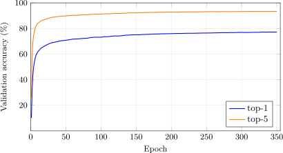
Why 420 epochs. The paper fixes the optimizer, the peak, the batch, the weight decay and the decay rate — \(\times 0.98\) per epoch — and leaves the length of the schedule unstated. The README’s command does not: about \(700\)K steps on eight clones of \(96\), which is \(700{,}000 \times 768 / 1{,}281{,}167 \approx 420\) epochs of data, with the stair every \(2.5\) epochs rather than every one. That staircase decays a fifth as often as the paper’s sentence, so at epoch \(420\) the rate is still \(0.12 \times 0.98^{167} \approx 4.1 \times 10^{-3}\), and the end-of-schedule polish a cosine run gets from annealing to zero comes here from the weight average at \(0.9999\) that the README scores instead. A run of \(90\) epochs under this recipe is a prefix of the same curve at a rate barely off its peak, which is why the validation tier is not the row; a shortened run has to substitute cosine to be worth anything, which is a different experiment rather than a cheaper version of the same one. Figure 6-3 is the check that the README’s length is enough. Table 6-2 is the run.

The wall-clock win over the \(6.2\times \)-larger ResNet-34 is real but sub-proportional, as §6.1 measured at small scale: depthwise convolution is memory-bound, so an order of magnitude fewer FLOPs buys a factor of two or three on this hardware rather than six. The RMSProp peak of \(0.12\) took off cleanly, because \(\varepsilon =1.0\) keeps the adaptive step well damped — in sharp contrast to EfficientNet’s \(\varepsilon =10^{-3}\) in Chapter 7. The last \(25\) epochs average \(71.72\% \), a tenth of a point under the endpoint. The paper’s figure is \(72.0\% \) and the README promises “roughly 72.0”; at \(n=50{,}000\) the Wilson 95% interval on this run is \([71.44, 72.23]\), so the README’s command is not distinguishable from the README’s number, which is the claim here and a weaker one than closing a gap by a measured amount.

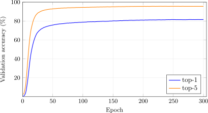
Epoch \(100\) has \(95\% \) of the final accuracy, the run is still climbing at \(200\), and the last \(50\) epochs move top-1 by \(0.37\) with the last \(25\) averaging a tenth under the endpoint: at the README’s length the curve is flattening, not flat, and the stair is still at \(4 \times 10^{-3}\), so this is where another hundred epochs stops being worth a day, not where the run stops moving.

The verified path (PJRT)

The verified trainer is apps/imagenette/MainMobileNetV2Imagenet.lean, built as lake build mobilenetv2-imagenet-verified, as the run below trained it:

-- Same inverted-residual backbone, 1000 classes instead of 10.
def mobilenetv2ImagenetVerified : VerifiedNetSpec where
  name       := "MobileNetV2 (ImageNet-1k)"
  slug       := "mobilenetv2in"
  data       := .imagenet
  shimScript := "generated_mobilenet_v2_imagenet_shim.py"
  layers     := [ ... the Imagenette stack, 1000-class head ... ]

-- 420 epochs at 64 PER DEVICE; four replicas give the global 256.
-- 420 because that is the README's ~700K steps of 768 at this batch.
def mobilenetv2ImagenetConfig : VerifiedConfig where
  epochs    := 420
  batchSize := 64
  bnMomentum := 0.997        -- TF-slim's BN decay, the reference's `bnMomentum`
  dwFanK2 := true            -- depthwise fan = k², as the JAX reference
  truncNormalSigma := 0.09   -- slim's truncated normal on every kernel

def main (argv : List String) : IO Unit :=
  mobilenetv2ImagenetVerified.toNet.trainAdamSched
    mobilenetv2ImagenetConfig (argv.head?.getD "data") ... variant

slug names verified_mlir/mobilenetv2in_<variant>_train_step.mlir, the rendered graph, and shimScript names this net’s own augmentation shim rather than ResNet-34’s — the shim the reference consumes, which is what makes the two a matched pair (§5-5). The head is the only parameter shape that moves, from \(1280 \times 10\) to \(1280 \times 1000\), which takes the count from 2.24M to 3,504,872 and matches the reference exactly. The BatchNorm layout is required to be byte-identical to the Imagenette net’s, and a #guard enforces it, because the running-stat region is positional and a drift there would misalign every frozen statistic at evaluation.

The variant carries the recipe. emarmstfdp64wxdwdoeps0001bf16 is the artifact the run below used, the reference’s recipe row for row: TF 1’s RMSProp (rmstf) at \(\rho = 0.9\), \(\mu = 0.9\), \(\varepsilon = 1.0\) with the rate inside the momentum term and the mean-square started at \(1\), coupled weight decay \(4 \times 10^{-5}\) off BatchNorm \(\gamma /\beta \), biases and the seventeen depthwise kernels (wx, dw), peak LR \(0.12\) with the \(\times 0.98\) staircase every \(2.5\) epochs from step \(0\) and no warmup, classifier dropout \(0.2\) (do), label smoothing \(0.1\), BatchNorm at TF-slim’s \(0.997\) / \(10^{-3}\) with the running statistics read at that \(\varepsilon \) by its eval graph mobilenetv2in_fwd_eval_eps0001, the weight average at \(0.9999\) in TF’s warmup-corrected form (ema, Theorem 88), which is what is scored, bf16 convolution under an fp32 classifier head, data-parallel over four replicas of \(64\) with each of the \(52\) BatchNorms all-reducing its mean and variance across them, so the statistic group is the global \(256\). Slim’s truncated-normal \(\sigma = 0.09\) is host-side, in the driver. The peak, the decay rate and the stair live in mnv2ImagenetRmsSchedule, which the driver reads, so the two paths cannot carry a different \(0.98\) or \(2.5\); the Imagenette peer’s mnv2RmsSchedule is the paper’s sentence, and the optimizer constants are mnv2RmsHyper. Theorem 94 ties this render’s bf16 gradient nodes to one device’s step at the global batch, its classifier dropout inside the statement. adam64 is AdamW at \(10^{-3}\) instead, the driver’s default because it matches the other ImageNet drivers. The job:

lake run mnv2-default-4gpu

Table 6-3 is the run.

The two paths, side by side

Table 6-4 is the two paths, row by row.

The BatchNorm group is held equal too: the reference normalizes over the global \(256\) under its mesh, and the verified render all-reduces to the same \(256\).

The two paths tie, \(-0.15\) on top-1 (77 images) and \(-0.01\) on top-5, inside the 95% Wilson interval (\(\pm 0.40\) at \(71\% \) on \(50{,}000\) images) at one seed each, and the curves sit on each other the whole way: the training losses agree to within \(0.005\) in every 25-epoch window, and the sampled accuracies never part by more than \(0.35\) at any epoch in the table. Paired on the same images, the two checkpoints agree on \(44{,}494\) and disagree on \(5{,}506\), \(2{,}792\) against \(2{,}714\), and McNemar’s exact test gives \(p = 0.30\): they cannot be told apart on this validation set. The pair this replaces ran the paper’s sentence rather than the README’s command — \(0.045\) unscaled with the stair every epoch for \(350\) epochs, no smoothing, no weight average, the depthwise kernels decayed, and on the verified side the depthwise init at the narrow fan and the head in a different precision from the reference’s — and read \(71.63\) against \(71.12\), a \(0.51\) gap with two of its rows held unequal; every row is held equal here by construction, and the gap is gone. Table 6-5 is the two paths at selected epochs and Figure 6-4 every ten.

What the MobileNetV2 recipe changes from the 2018 recipe

The ResNet-34 trainer of Chapter 5 is the 2018-era recipe of the SGD lineage: momentum, cosine polish, label smoothing. MobileNetV2 is a 2018 paper too, but from the other side of a fork. Google’s TensorFlow and Inception training tradition runs RMSProp with a huge \(\varepsilon \), an exponential LR staircase, a tiny weight decay, and nothing beyond crop and flip on the data side. So this diff is not a time jump but two contemporary recipes side by side, and it is the base that the next chapter’s 2019 EfficientNet recipe is built on. The entry point is the same on both paths, and every row of Table 6-6 is one argument or one field:

What carries over unchanged: batch 256, train and eval both at \(224\), running-BN evaluation, and bf16 convolution under an fp32 classifier head. R34’s 5-epoch warmup does not: MobileNetV2’s staircase starts at step \(0\), as the paper’s does.

The through-line of this fork is that nothing here regularizes harder. MobileNetV2’s recipe is the SGD recipe’s contemporary, tuned for a network \(1/6\) the size, and its distinctive knobs (adaptive optimizer, staircase decay, a tiny weight decay on the kernels alone, the weight average) are the ones EfficientNet inherits and ConvNeXt eventually replaces wholesale. The 2019–2022 tables that follow all diff against the same 2018 SGD column. This one shows where their other half came from.

The general pattern is deeper and narrower, with a per-channel conv between surrounding \(1 \times 1\) expansions, and it carries forward to MobileNet V3 and the EfficientNet family. All of those add their own small modifications on top (SE blocks, Swish activations, compound scaling) but the core depthwise-separable scaffolding is exactly what this chapter formalized.

6.6 Side quest: MobileNet V4

Six years on, MobileNetV4 (Qin et al. 2024, arXiv:2404.10518) revisits this chapter’s block. Its central move is the universal inverted bottleneck (UIB): take the inverted residual and make two depthwise positions optional, one before the expansion and one after it. Four instantiations fall out of that one template. Both depthwise convs on is ExtraDW. Only the leading one is ConvNeXt, this chapter’s sandwich rearranged into Chapter 8’s block shape. Neither is a plain FFN of two \(1\times 1\)s. Only the inner one is exactly MobileNetV2’s block. The jax/ folder ships the faithful Conv-Medium as a full ImageNet trainer (jax/MainMobilenetV4Imagenet.lean), transcribed block for block from timm’s mobilenetv4_conv_medium and tied to it on shared weights (scripts/parity/mnv4_timm_parity.py, to \(\sim \! 10^{-5}\) in the training forward): \(9{,}715{,}512\) parameters, a fused-IB stage at high resolution, then 21 UIB blocks whose per-block instantiation is visible right in the NetSpec, driven by the same entry point as every other net in this book. What changed from 2018 to 2024 is at least as much recipe as architecture, and Table 6-7 is the diff.

The direction of travel matches the recipe tables of Chapters 7 and 8: by 2024 the mobile lineage has converged on the same transformer-era training recipe as everything else (AdamW at large effective batch, cosine, heavy selective decay, RandAugment, EMA) while the block template generalized enough to absorb its rivals.

mobilenet-v4-imagenet ships the paper recipe as full, and a detuned 100-epoch tier as default (\(224\), the regularization turned down, an EMA shadow) for a short run; the paper tier is what this section reports. The paper’s recipe is a training config in tensorflow/models (imagenet_mobilenetv4_conv_medium_tpu.yaml), and full is that file: \(256^2\) input, weight decay \(0.1\) off the norms and biases, classifier dropout \(0.2\), RandAugment \(N2\) \(m15\) at \(p\, 0.7\) under TensorFlow’s own mappings (nearest resampling, fill \(128\), the identity op in the draw), drop-path \(0.075\) ramped as \((i+3)/26\) over the block list and applied at the 18 UIBs that carry a skip, BatchNorm at decay \(0.997\) and \(\varepsilon = 10^{-3}\), AdamW at Keras’ \(\varepsilon = 10^{-7}\), the cosine from step \(0\) with the five-epoch warmup on top, tf-models’ crop sampler with its centre-crop fallback and its bilinear resize without antialiasing, and no EMA, so the live weights are what gets scored, at the paper’s \(256\) with a \(0.875\) centre crop. The yaml says \(500\) epochs, and the \(79.9\% \) headline is that number. The pair this section is built on is that recipe with only the length cut, to \(100\), on both paths. Everything the recipe asks of the code is exercised by it; the 500-epoch run is the same two jobs with a longer cosine, and it is the one thing here that has not run.

The reference (JAX)

The reference trainer is jax/MainMobilenetV4Imagenet.lean, built as lake build mobilenet-v4-imagenet, with .imagenet streamed through tfds; its job config is scripts/jobs/mnv4-full100-jax-4gpu.conf, recipe full100, which is the full config with epochs := 100: the generated trainer differs from full’s in one constant and the shim is byte-identical. AdamW at peak \(0.004\) for an effective batch of \(4096\), reached as a \(512\)-image micro-batch accumulated eight times, so \(312\) optimizer steps an epoch; bf16 convolutions against fp32 master weights; the live weights scored every fifth epoch and the last, through an fp32 forward. Table 6-8 is the run.

The trainer is feed-bound at this shape, \(2.55\) s an optimizer step with the four cards waiting on the input pipeline. It restarted once: a corrected PCIe error on the chipset’s upstream bridge, not a GPU, at epoch 48, which the supervisor’s AER policy treats as a kill; it resumed from the epoch-47 checkpoint twenty seconds later and lost about ten minutes. Set against this chapter’s other half, that is the six-year argument in two rows: \(\mathbf{+5.55}\) points over MobileNetV2’s README-faithful \(71.84\% \), from \(2.8\times \) the parameters and under a quarter of the epochs, \(100\) against \(420\). By 2024 the mobile line is not trading accuracy for size so much as reaching the same accuracy with a block that happens to be cheap. Figure 6-5 is the run, scored every five epochs.

The last ten epochs move top-1 by \(0.49\) (\(76.90 \to 77.33 \to 77.39\)), so at a hundred epochs this schedule is not exhausted: the pack wants the length, which is what the yaml’s \(500\) is for, and the \(2.5\) points to \(79.9\% \) are the schedule’s to close.

The verified path (PJRT)

The spec follows §6-3 and §5-5. The trunk is copied unchanged from the Imagenette spec, a #guard pins every parameter shape but the head against it, and the head moves \(1280{\times }10 \to 1280{\times }1000\), taking the count from \(8{,}447{,}322\) to \(\mathbf{9{,}715{,}512}\), the reference’s count exactly:

def mnv4ImagenetVerified : VerifiedNetSpec where
  name       := "MobileNetV4-Conv-M (ImageNet-1k)"
  slug       := "mnv4in"
  imageH     := 224
  imageW     := 224
  data       := .imagenet
  shimScript := "generated_mobilenet_v4_imagenet_shim.py"
  layers     := [
    .convBnNB 3 32 3 2,               -- stem                       224->112
    .fusedMbConvNB 32 48 4 3 2,       -- stage 0, fused IB          112->56
    .uib  48  80 4 2 3 5,             -- ... the Imagenette UIB stack, 21 blocks
    .convBnNB 256 960 1 1,
    .globalAvgPool,                   -- timm pools BEFORE conv_head
    .convBnNB 960 1280 1 1,
    .dense 1280 1000 ]                -- 1000-class head
  runningBN   := true
  dropoutKeep := some (0.9, 1280)     -- classifier dropout 0.1, for the `do` variants

-- The head is the ONLY thing that may differ from the 10-class net.
#guard mnv4ImagenetVerified.toSpecs.size == mobilenetv4Verified.toSpecs.size
#guard mnv4ImagenetVerified.toSpecs.pop.pop == mobilenetv4Verified.toSpecs.pop.pop
#guard mnv4ImagenetVerified.toSpecs.back!  == (#[1000], 2)
#guard mnv4ImagenetVerified.bnChannels == mobilenetv4Verified.bnChannels

That is apps/imagenette/MainMobilenetV4Imagenet.lean. It builds as mobilenetv4-imagenet-verified. The renders come from the same chain and the same block table as the three 10-class artifacts, differing only in the head, the batch and the slug, which is why adding them was three #eval lines rather than a new proof chain. The inference graphs, mnv4in_fwd_eval and mnv4in_fwd_eval_s256, denote the frozen-statistics forward at any final feature size (mnv4FwdGraphBFullEval_faithful), and their block text is pretty of the typed graph at both sizes (FwdGraphTextTies); the classifier-dropout forward is stated at every mask and at either precision (mnv4FwdGraphBFullDo_faithful).

The paper tier is that spec with three host-side fields moved and, at the paper’s \(256\), a slug of its own:

def mnv4Imagenet256FullVerified : VerifiedNetSpec :=
  { mnv4ImagenetFullVerified with      -- full shim (m15), dropout 0.2, 18 drop sites
      name          := "MobileNetV4-Conv-M (ImageNet-1k, paper tier, 256²)",
      slug          := "mnv4in256",
      imageH        := 256,
      imageW        := 256,
      dropDenom     := 26,              -- tf-models: UIB i keeps 1 - 0.075 (i+3)/26
      dropIdxOffset := 3,
      ... }                             -- the blurb

#guard mnv4Imagenet256FullVerified.toSpecs == mnv4ImagenetVerified.toSpecs

That is LeanMlir/Verified/NetsCore.lean: the same layers and the same parameter shapes, with the shim swapped for the full recipe’s, the classifier dropout at the paper’s \(0.2\), and stochastic depth reaching the 18 skip UIBs at tf-models’ ramp over its 26-entry block list. The mnv4in256 renders come off the same chain and the same block table as mnv4in’s, at final side \(8\) instead of \(7\).

The variant carries the recipe. mnv4in256_accdp8x128wxdropdowd01bf16 is the artifact the run used: AdamW at \(0.004\), four replicas of \(128\) accumulated eight times to the reference’s effective \(4096\), drop-path and classifier dropout in the graph, weight decay \(0.1\) with the norms and biases excluded, bf16 convolution under an fp32 classifier head, BatchNorm \(\varepsilon \, 10^{-3}\) and AdamW \(\varepsilon \, 10^{-7}\) baked. Each of the 77 BatchNorms all-reduces its mean and variance across the four replicas, so the statistic group is the \(512\)-image micro-batch, which is the group the reference’s accumulation gives it. Theorem 95 ties the data-parallel render’s bf16 gradient nodes to one device’s step at the global batch, and is stated at \(224^2\): the \(256^2\) render has not had it restated, so on this pair the data-parallel step is the render’s and not a theorem’s, and accumulation and the two dropouts sit outside the statement as before. Disclosed, on both paths: the initialization is timm’s, and the decay reaches the classifier bias. It runs with:

lake run mnv4-full-e100-4gpu

LEAN_MLIR_EPOCHS=100 sets the cosine as well as the loop bound, under the run’s own checkpoint tag. Table 6-9 is the run.

Compute-bound at \(214\) ms a micro-step, which is why the proven graph finishes six and a half hours ahead of the Python trainer on the same four cards; no restart and no thermal rest.

The two paths, side by side

Table 6-10 is the two paths, row by row.

Above the rule, beside the lowering, sit the precision of the classifier head and the depthwise initialization, which starts every depthwise kernel \(\sqrt{C}\) narrower on the verified path.

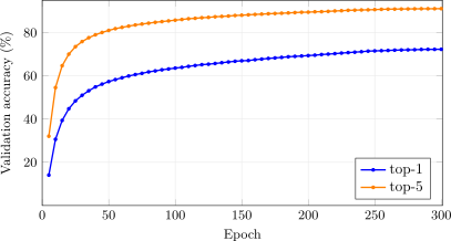
The pair ties. \(-0.04\) on top-1 and \(+0.07\) on top-5 are a tenth of one run’s \(\pm 0.37\) Wilson half-width at \(n = 50{,}000\), and the curves cross back and forth the whole way: at epoch 60 the two score \(34{,}753\) and \(34{,}750\) images correct, and the means of the last five scored epochs are \(76.56\) and \(76.60\). Table 6-11 is the selected epochs and Figure 6-6 every five. The McNemar pairing of §5-5 is owed: only the verified trainer writes the per-image bitmap, and the reference’s checkpoint is kept for the rescore that produces its half.

[TODO: the schedule, and what the pair above still owes the paper’s own code. The same two jobs at \(500\) epochs, mnv4-full-jax-4gpu / mnv4-full-4gpu, \({\sim }112 + 78\) h on the 4060 Ti box, this pair times five, are owed. The \(100\)-epoch pair above predates two rows of that recipe, on both paths: the stochastic-depth ramp over tf-models’ \(26\)-entry block list (the gpooling row counts; the pair ran \(/25\)), and tf-models’ centre-crop fallback where the crop sampler returns the whole image (the pair fell back to the whole image). Still out, disclosed on both paths: the initialization (tf-models draws every convolution and depthwise kernel from Keras’ VarianceScaling, fan-in, truncated normal, and the classifier \(U(\pm 0.05)\); ours is timm’s), weight decay reaching the classifier bias (the yaml exempts BatchNorm alone; ours exempts every bias), and the BatchNorm group (per TPU core there, the \(512\)-image micro-batch here). What the pair does not owe: the head order is tf-models’ too (its block list pools before the \(1280\) convolution).]

6.7 Recap

Depthwise convolution is the standard convolution with the channel sum removed, one kernel per channel, and its backward is two convolutions of its own: an input VJP built from \(\operatorname {pdiv}\), and a weight gradient, each proved at stride one and two. ReLU6 is ReLU with a ceiling. With those two the whole MobileNetV2 is proved at all seventeen blocks and MobileNetV4 at full depth (Theorems 82 and 83), both steps are tied and both have their data-parallel twins. On ImageNet the chapter runs two generations of the same block, and the recipe table between them is six years of training practice in one page: by 2024 the mobile line trains the way everything else does.

What is open is the schedule: the paper tier ran at a hundred epochs on both paths and tied, and its five hundred are the one job in the chapter that has not. The next block keeps the depthwise convolution and adds a gate around it, a learned per-channel gain computed from the map itself, which is the third composition rule, multiplicative fan-in, and the first attention mechanism in the book. Its activation is smooth, and that changes what the theorems can say.