7 EfficientNet
A convolution treats every channel equally
By the time a feature map reaches a deep stage of a CNN, each channel is a learned “feature detector” for something specific: a headlight, a curve, a fur texture, a leaf edge. A standard \(3 \times 3\) convolution that consumes this feature map treats every one of those channels as equally important contributors to every output channel. Its kernel learns a fixed mixing recipe that’s applied to every spatial position of every input image, regardless of what’s actually in the image.
That’s wasteful in a particular way. A “headlight” channel is useful when there’s a car in the image and useless on a beach. A “leaf-edge” channel is useful in a tree-heavy region and useless in the sky. The network has no built-in way to say “for this image, dial channel 47 up and channel 112 down.” Hu et al. 2018 (arXiv:1709.01507) designed a tiny module that lets the network do exactly that: look at the global content of the feature map, produce a per-channel gain, and rescale every channel by its gain before passing the feature map forward.
That module is the Squeeze-and-Excitation block, and at its core it is a learned per-channel attention mechanism, contemporary with the transformer’s (Vaswani et al. 2017) and three years ahead of attention’s arrival in vision.
7.1 Run it first
Before the attention mechanism, train the network that uses it. Four commands, and about forty minutes of GPU time:
lake exe cache get                            # Mathlib oleans, ~30 s
./scripts/datasets/download_imagenette.sh     # 330 MB dl, 2.4 GB unpacked
lake build efficientnet-verified-adam
./.lake/build/bin/efficientnet-verified-adam data
On one RTX 4060 Ti (CUDA 12.9), from runs/2026-08-12-enet-imagenette-xla-cuda/. XLA’s startup banner is removed, the network description line is wrapped, and the middle of the run is elided:
[pjrt_ffi] XLA backend: PJRT 0.112, 1 device(s)
[pjrt_ffi] compiled verified_mlir/efficientnet_adam_train_step.mlir
             (@efficientnet_adam_train_step, 740 outputs, 1 replica)
             in 10603 ms
[pjrt_ffi] compiled verified_mlir/efficientnet_fwd.mlir
             (@efficientnet_fwd, 1 outputs, 1 replica) in 635 ms
[pjrt_ffi] compiled verified_mlir/efficientnet_fwd_eval.mlir
             (@efficientnet_fwd_eval, 1 outputs, 1 replica) in 454 ms
EfficientNet-B0 on Imagenette 224² (stem-s2 → 16 MBConv [t,c,n,s,k],
  swish + squeeze-excite + batch-norm, 5 downsamples 224→7 →
  head 320→1280 → GAP → dense)
  via the VERIFIED renderer → XLA/PJRT → GPU
  train 9469, val 3925; bs 32, EfficientNet-B0 adam
    (cosine+warmup 3ep, baseLR 0.001000), He init
  running-stats BN: 49 layers, 42016 stat floats
    → eval via @efficientnet_fwd_eval
Epoch 1/80: loss=2.063774 lr=0.000333
  epoch 1: val_acc = 758/3925 = 19.312102%  top5 = 2630/3925 = 67.006369%
Epoch 2/80: loss=1.631765 lr=0.000667
  epoch 2: val_acc = 1216/3925 = 30.980892%  top5 = 2889/3925 = 73.605096%
Epoch 3/80: loss=1.430369 lr=0.001000
  epoch 3: val_acc = 1526/3925 = 38.878981%  top5 = 3173/3925 = 80.840764%
Epoch 4/80: loss=1.294553 lr=0.001000
  epoch 4: val_acc = 2116/3925 = 53.910828%  top5 = 3521/3925 = 89.707006%
Epoch 79/80: loss=0.504706 lr=0.000000
  epoch 79: val_acc = 3535/3925 = 90.063694%  top5 = 3857/3925 = 98.267516%
Epoch 80/80: loss=0.505049 lr=0.000000
  epoch 80: val_acc = 3534/3925 = 90.038217%  top5 = 3858/3925 = 98.292994%
done (trained EfficientNet-B0 adam + cosine/warmup via packed threading).
Eighty epochs at about 30 seconds each, forty-one minutes in total, and 90.04% top-1 with 98.29% top-5 on Imagenette’s 3,925-image validation split. The best epoch reached \(90.17\% \). That is level with ResNet-34’s five-seed \(89.99 \pm 0.32\) and eight tenths of a point over MobileNetV2’s \(89.25\% \), on the same data, the same recipe and the same eighty epochs. EfficientNet-B0 does it with \(5.3\times \) fewer parameters than ResNet-34 and in forty-one minutes against forty-seven.
The first four epochs are worth a glance. Top-1 climbs 19.3, 31.0, 38.9, then jumps to 53.9. The learning rate is still warming up through epoch 3, and the BatchNorm running statistics are averaging over weights that are moving fast, so the evaluation forward is using statistics that no longer describe what is being evaluated. It resolves once the schedule reaches its peak and never recurs.
Squeeze-excitation is the first place the product rule carries real weight. As in Chapter 6, what ran is pretty(provenGraph) — verified_mlir/efficientnet_adam_train_step.mlir — and every squeeze-excitation gate in it backpropagates by the product rule Theorem 86 proves; the depthwise, BatchNorm and residual rules are Theorems 71, 49 and 58.
And this fold holds at every input. efficientnetForwardBFullHasVJP chains the stem, all sixteen MBConv blocks and the head through vjpComp, batched over \(N\), assuming a positive \(\varepsilon \) at each BatchNorm and nothing else — so every operation in the graph that just trained carries a proved backward, and their composition into the whole network carries one too. What buys that is swish. It is smooth, so the statement quantifies over all inputs, where Chapter 6’s fold had to name a point and assume every relu6 activation stayed off the kink. Depth was never the obstacle, the activation was — and every network after this one is smooth.
The three compile lines and the running-stats BN line are every BatchNorm net’s, here at 49 BatchNorms; the train step’s 740 outputs are what 213 parameter tensors plus their Adam moments plus the batch statistics plus the report-only loss come to.
Three steps, one tensor product
An SE block on a feature map \(x \in \mathbb {R}^{B \times C \times H \times W}\) runs three operations in sequence:
Squeeze. Global-average-pool across spatial dimensions: \(s_c = \frac{1}{HW} \sum _{i,j} x_{c, i, j}\). Result is a \(B \times C\) tensor: one scalar per image per channel, summarizing the channel’s overall activity.
Excite. Push \(s\) through a tiny two-layer MLP with a bottleneck: \(g = \sigma (W_2\, \mathrm{ReLU}(W_1 s))\), where \(W_1\) is \(C \to C/r\) and \(W_2\) is \(C/r \to C\) for a reduction ratio \(r\) (typically 16). The sigmoid squashes each output to \([0, 1]\). Result: \(g \in \mathbb {R}^{B \times C}\), a per-channel gate value.
Apply. Multiply the original feature map by the gates, broadcast across the spatial axes: \(y_{c, i, j} = g_c \cdot x_{c, i, j}\). Channels with gate near 1 pass through, and channels with gate near 0 are suppressed.
That’s it. The MLP operates on a \([B, C]\) tensor, not \([B, C, H, W]\), so it’s tiny, at \(C^2 / r + C/r + C\) parameters per block against millions for a standard conv at the same width.
From the framework: it’s an elementwise product
What is the SE block, as a function? Up to a learned scalar factor per channel, it’s just an elementwise product of the input with a side branch:
where the gate \(g\) is built from the saved input \(x\) via two dense layers and a sigmoid. We already proved the VJP of an elementwise product (Theorem 12). We already proved the VJP of dense (Theorem 18). We already proved the VJP of identity, and an additive fan-in collapses to the same product-rule structure as elementwise. Theorem 86 is one line of composition, and it introduces no new analytic dependencies.
Attention in Disguise
SE looks at the entire feature map, produces a content-dependent re-weighting, and applies it back to the data. That is a learned attention operation in the standard sense. The reduction is over the spatial axes (so each token-equivalent is a channel, not a patch), but the shape is the same: a query (GAP summary) attending over a collection (the channels) to produce weights, weights gating the original signal.
The transformer’s self-attention (Vaswani et al. 2017) generalizes the same pattern from a fixed query (the GAP) to a learned sequence of queries (the token positions) and from a fixed key/value (the channels) to a learned key/value (per-token features). SE is the bare minimum version of that idea. Most post-2018 convolutional architectures carry SE or one of its descendants (CBAM, ECA, GE), because the accuracy-per-parameter cost is low and the operation composes cleanly with anything else.
EfficientNet-B0: MobileNet-V2 with SE everywhere
EfficientNet-B0 (Tan & Le 2019, arXiv:1905.11946) is, at the architectural level, MobileNet-V2 with two changes:
Every MBConv block contains an SE sub-module after the depthwise conv. The verified spec spells that as its own constructor, .mbConvSENB, rather than as a flag.
Swish (\(x \cdot \sigma (x)\)) replaces ReLU as the activation. Smoother gradient, modest empirical lift, and no new VJP structure, just chain rule through a sigmoid.
The paper’s actual thesis is compound scaling: jointly scale depth, width, and input resolution by a single coefficient \(\phi \) and you get the EfficientNet family B0 through B7, with B7 reaching ImageNet state-of-the-art at the time. At the B0 baseline (the one in this book), the architectural lift over MobileNet-V2 is essentially SE plus Swish. The compound scaling story lives in the B0\(\to \)B7 progression, which we don’t fit on Imagenette because the dataset is too small for the return-on-scaling to show up.
7.2 The theorems
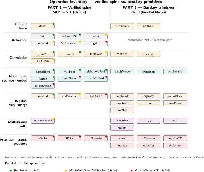
assume:
\(B_g\) is a correct backward function for the gate (\(\mathsf{HasVJP}\, \mathrm{gate}\)) [hg]
\(\mathrm{gate}\) is differentiable everywhere [hg_diff]
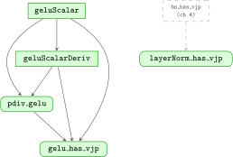
prove: \(\mathsf{HasVJP}\, (\mathrm{seBlock}\, \mathrm{gate})\), where \(\mathrm{seBlock}\, \mathrm{gate}\, x = x \odot \mathrm{gate}(x)\), with backward
SE multiplies input by a sigmoid-gated channel mask.
\(\mathrm{seBlock}\, \mathrm{gate} = \mathrm{elemwiseProduct}\, \mathrm{id}\, \mathrm{gate}\).
proof: Definitional.q.e.d.
proof: Instantiate the multiplicative fan-in VJP (Theorem 12) at \(f = \mathrm{id}\) (differentiable; its VJP is Theorem 13), with assumptions 1 and 2 supplying the gate side. The general backward \(B_f(x, g(x) \odot dy) + B_g(x, f(x) \odot dy)\) specializes: the identity’s backward passes \(\mathrm{gate}(x) \odot dy\) through unchanged (main path, each channel scaled by its gate), and the gate sub-network sees \(x \odot dy\) as its cotangent — not bare \(dy\).
The ladder for EfficientNet-B0: the VJP, the chain, the step, the loss gradient and the data-parallel tie; no seal.
assume:
every BatchNorm’s \(\varepsilon {\gt} 0\), forty-nine of them [h\(\varepsilon \)w]
prove: the backward composed from the per-block backwards, for the batched EfficientNet-B0 — sixteen MBConv blocks with squeeze-and-excitation and swish, at training BatchNorm and batch \(N\) (efficientnetForwardBFull) — equals the \(\operatorname {pdiv}\)-contracted Jacobian of the forward at every input, cotangent and pixel; and the emitted forward graph denotes exactly that forward. With stochastic depth on the nine blocks that carry a skip and classifier dropout between the pool and the dense, the drop and dropdo forward graphs denote the masked forward at every mask, at training and at inference BatchNorm, in f32 as the committed efficientnetin_drop_fwd and efficientnetin_dropdo_fwd are. There is no smooth-point hypothesis: swish and the SE gate have no kink.
A fold of the VJP chain rule (Theorem 10) over the stem, the sixteen blocks (Theorems 58 and 86) and the head; the graph ties op by op; see Proofs.efficientnetForwardBFullHasVJP_correct.
assume:
every BatchNorm’s \(\varepsilon {\gt} 0\) [h\(\varepsilon \)w]
prove: the hand-written sixteen-block reverse chain efficientnetInputGradBFull equals
for every batch, cotangent and pixel.
The chain is the composed backward of Theorem 87 read stage by stage; see Proofs.efficientnetInputGradBFull_correct.
prove: each of the 213 emitted parameter gradients of the batched EfficientNet-B0 step (efficientnet_adam_train_step.mlir and the efficientnetin_* steps) denotes the certified batch gradient at the chain cotangent of the label-smoothed cross-entropy — through swish, the SE gate’s fan-in and the batch-BatchNorm backward — with the target and the number of classes binders. Stated at one replica, at either precision, with stochastic depth on the nine skip-carrying blocks and the classifier dropout as optional masks: at none the chain is the drop-free artifacts’, at some the drop, do and dropdo renders’ — efficientnetin_emarmsdp64dropdowxeps0001bf16 among them — where a masked block’s nodes read the cotangent through its site and the skip reads it raw, and the dense weight node reads the dropped activation; the optimizer tails that consume the nodes are outside it.
A fold over the 213 nodes, the chain’s cotangents the certified block backwards; see Proofs.EnetTieG.efficientnet_net_tiedG.
assume:
every BatchNorm’s \(\varepsilon {\gt} 0\) [h\(\varepsilon \)w]
\(L\) is any loss of the logits, with gradient \(g\) there [hL]
prove: for each node of Theorem 89, the node at the chain cotangent from \(g\) is \(\partial L/\partial \theta \) of the forward at the same masks (efficientnetForwardBFullDrop; efficientnetForwardBFull at none) with that one parameter varied, at any batch and number of classes. Instantiated at the label-smoothed cross-entropy.
The step tie’s node, with \(g\) pulled back through the certified block backwards (Theorem 15, once per stage); see Proofs.EnetTieG.enet_net_lossGrad.
assume:
\(R \ge 1\) replicas of \(N \ge 1\) images each, all forty-nine BatchNorms synchronised with \(\varepsilon {\gt} 0\) [hR, hN, h\(\varepsilon \)w]
each replica’s loss cotangent is its shard of the global batch’s, scaled by \(R\) [hgs]
prove: the mean over replicas of each of the 213 all-reduced gradient nodes of the data-parallel renders at either precision (efficientnetin_emarmsdp64dropdowxeps0001bf16 among them, at \(\texttt{replicas} {\gt} 1\); loss \(\div B\) per replica; each replica’s stochastic-depth and dropout masks the shards of global ones) equals the single-device node of Theorem 89 at batch \(R \cdot N\) and those global masks, loss \(\div (R \cdot B)\). Instantiated at the label-smoothed cross-entropy.
With synchronised statistics a replica’s forward is the global forward on its shard, so its node is the global node’s sum over that shard, scaled by \(R\); the mean of the \(R\) shard sums is the global sum; see Proofs.EnetSyncTieG.efficientnet_net_syncTiedG.
7.3 Example: EfficientNet-B0 on Imagenette
The architecture
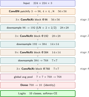
EfficientNet-B0 is the MobileNetV2 column with Squeeze-and-Excitation in every block: the same \(3 \times 3\) stride-2 stem, seven stages of MBConv blocks (kernel sizes mixing \(3 \times 3\) and \(5 \times 5\) depthwise), the \(1 \times 1\) lift to 1280, global average pool, and dense head. The inset shows one MBConv block, an inverted residual with an SE gate (highlighted) inserted before the project.
--(\b);
\foreach \n/\k in {m1/1,m2/2,m3/3,m4/4,m5/5,m6/6,m7/7}\node[stage] at ($(\n.east)+(0.30,0)$){stage \k};
\end{tikzpicture}](images/img-0035.svg)
--(\b);
\draw[skip] (x.north) .. controls +(0,0.9) and +(0,0.9) .. (sum.north)
node[midway, above, term, magenta!70!black]{skip if stride 1, $C_{\text{in}}{=}C_{\text{out}}$};
\node[term, below=0.16cm of s, gray!55!black]{one MBConv block: inverted residual $+$ squeeze-excitation};
\end{tikzpicture}](images/img-0036.svg)
The verified trainer
The pattern is §5.3’s; only the layers list and the bnChannels that follows from it are new:
import LeanMlir.Verified.NetsCore
import LeanMlir.Verified.Train

-- 1. The network. `slug` names the committed render, `bnChannels`
--    drives BN threading, `NB` means the BN-followed convs carry
--    no bias.
def efficientnetVerified : VerifiedNetSpec where
  name     := "EfficientNet-B0"
  slug     := "efficientnet"
  inC      := 3
  imageH   := 224
  imageW   := 224
  data     := .imagenette
  layers   := [
    .convBnNB 3 32 3 2,             -- stem 3x3-s2   224->112
    .mbConvSENB  32   32  16  8 3,  -- stage 1, t=1 (no expand)
    .mbConvSENB  16   96  24  4 3,  -- stage 2       112->56
    .mbConvSENB  24  144  24  6 3,
    .mbConvSENB  24  144  40  6 5,  -- stage 3        56->28
    .mbConvSENB  40  240  40 10 5,
    .mbConvSENB  40  240  80 10 3,  -- stage 4        28->14
    .mbConvSENB  80  480  80 20 3,
    .mbConvSENB  80  480  80 20 3,
    .mbConvSENB  80  480 112 20 5,  -- stage 5           @14
    .mbConvSENB 112  672 112 28 5,
    .mbConvSENB 112  672 112 28 5,
    .mbConvSENB 112  672 192 28 5,  -- stage 6        14->7
    .mbConvSENB 192 1152 192 48 5,
    .mbConvSENB 192 1152 192 48 5,
    .mbConvSENB 192 1152 192 48 5,
    .mbConvSENB 192 1152 320 48 3,  -- stage 7            @7
    .convBnNB 320 1280 1 1,         -- head, 1x1 to 1280
    .globalAvgPool,
    .dense 1280 10 ]
  bnChannels := #[32, 32,16, 96,96,24, ... ]  -- all 49, in order

-- 2. The schedule. ResNet-34's and MobileNetV2's, unchanged.
def efficientnetAdamConfig : VerifiedConfig where
  epochs    := 80
  batchSize := 32

-- 3. The entry point: AdamW, cosine with a 3-epoch warmup, baseLR 1e-3.
--    The rms variant, the EMA decay and the drop rate are env knobs.
def runEfficientNetAdam (argv : List String) : IO Unit := do
  let variant := (← IO.getEnv "LEAN_MLIR_VARIANT").getD "adam"
  let bs := ((← IO.getEnv "LEAN_MLIR_BATCH").bind (·.toNat?)).getD
              efficientnetAdamConfig.batchSize
  let sched := enetRmsSchedule
  let rms := variant.contains "rms"
  let baseLR := match (← IO.getEnv "LEAN_MLIR_BASE_LR_U").bind (·.toNat?) with
    | some u => u.toFloat * 1e-6
    | none   => if rms then sched.lr * bs.toFloat / 256.0 else 0.001
  let emaDecay := match (← IO.getEnv "LEAN_MLIR_EMA_DECAY_U").bind (·.toNat?) with
    | some u => u.toFloat * 1e-6
    | none   => 0.9999
  let dropNet := match (← IO.getEnv "LEAN_MLIR_DROP_RATE_U").bind (·.toNat?) with
    | some u => { efficientnetVerified.toNet with
                  dropKeeps := efficientnetVerified.dropKeepsAt (u.toFloat * 1e-6) }
    | none   => efficientnetVerified.toNet
  dropNet.trainAdamSched { efficientnetAdamConfig with batchSize := bs }
    (argv.head?.getD "data") baseLR 0.9 0.999 3 variant
    (if rms then sched.decayRate else 0.0) sched.decayEpochs emaDecay
def main (argv : List String) : IO Unit := runEfficientNetAdam argv
.mbConvSENB ic mid oc r k is one block per line, as Chapter 6’s constructor was, with mid the expanded width; k is the depthwise kernel, mixing \(3 \times 3\) and \(5 \times 5\) by stage, and the expand \(1 \times 1\) is skipped exactly when mid == ic, which is stage 1 and its \(t=1\).
r is the squeeze width, and it is sized off ic. Every block in the listing has r == ic/4: 32 gives 8, 16 gives 4, 192 gives 48. That is the correctness note this chapter returns to in §7.5 from the other direction, and it is worth reading here first, because sizing the squeeze off the \(6\times \)-larger mid instead is the difference between B0’s canonical 5.29M parameters and an inflated 8.4M. The spec is where that choice is made once and visibly.
The arm, and where the SE gate lives in it.
  | mbConvSENB ic mid oc r k =>                -- Ch. 7
    (if mid != ic then #[(#[mid,ic,1,1],0),(#[mid],1),(#[mid],2)] else #[])
    ++ #[(#[mid,1,k,k],0),(#[mid],1),(#[mid],2),     -- depthwise kxk + BN
         (#[mid,r],0),(#[r],2),(#[r,mid],0),(#[mid],2),   -- SE: squeeze, excite
         (#[oc,mid,1,1],0),(#[oc],1),(#[oc],2)]     -- project 1x1 + BN
Same mid != ic conditional as Chapter 6’s, with four tensors inserted in the middle: [mid,r] down to the squeeze width and [r,mid] back up, each with a bias. Those two are the only convs in the block that keep their biases, because they are not BN-followed — the gate ends in a sigmoid, not a normalizer. That asymmetry is visible in the arm and nowhere else in the spec.
There is no stride argument, and that is deliberate. B0’s downsampling pattern is fixed by the architecture rather than chosen per block, so it lives in the renderer, which emits b1 as no-expand, b2, b4, b6 and b12 as strided, and the remaining nine as residual. The spec’s job is the parameter layout, and efficientnetVerified.toSpecs is kernel-#guarded against an independently audited hand-list.
The BatchNorm list has 49 entries, not the 50 a per-block count gives. Every MBConv normalizes after its expand, depthwise and project convs, which would be \(16 \times 3 + 2\) for the stem and head, or 50. Stage 1 has \(t=1\) and therefore no expand conv, so it contributes two entries rather than three, and the real count is 49. bnChannels exists to get that right: the running-stat region is positional, and an off-by-one misaligns every frozen statistic downstream of it at evaluation time.
The squeeze-excite biases stay. NB drops the bias from every convolution a BatchNorm follows, because the BatchNorm’s own shift absorbs it. SE’s two \(1 \times 1\)s are followed by a sigmoid gate rather than a BatchNorm, so nothing absorbs theirs and they are kept. The rule is about what comes after a convolution, not about the convolution.
Every SE block multiplies the input by the sigmoid output of its two-layer MLP: that is exactly Theorem 86 composed with Theorem 12 and the dense VJP (Theorem 18). No new math in this chapter beyond the SE block itself.
Results
§7.1 has the run: 80 epochs at about 30 seconds each, forty-one minutes, \(\mathbf{90.04\% }\) top-1 and \(\mathbf{98.29\% }\) top-5, with the loss settling on the same \({\sim }0.50\) label-smoothing floor as ResNet-34 and MobileNetV2. The three-chapter comparison — same dataset, same recipe, same eighty epochs, and every row now a measurement on the verified XLA path, on one RTX 4060 Ti:
|
Model |
Params |
MLIR |
Step time |
Total |
Top-1 |
Top-5 |
|
ResNet-34 |
21.29M |
754 KB |
120 ms |
47 min |
89.99% |
98.46% |
|
MobileNetV2 |
2.24M |
1,071 KB |
90 ms |
35 min |
89.25% |
98.68% |
|
EfficientNet-B0 |
4.02M |
1,317 KB |
103 ms |
41 min |
90.04% |
98.29% |
Step time is the epoch wall-clock divided by 295 batches, so it includes each epoch’s validation pass. MLIR sizes are the committed <slug>_adam_train_step.mlir in 1000-byte units. ResNet-34’s accuracies are the five-seed means of §5.6 (runs/2026-09-12-r34-ablation-fp32-seeds/) and its times are one of those seeds’ (§5.1); the other two rows are one run each.
EfficientNet-B0 is level with ResNet-34 on top-1, at \(90.04\% \) against \(89.99 \pm 0.32\), and eight tenths of a point over MobileNetV2’s \(89.25\% \). It gets there with \(5.3\times \) fewer parameters than ResNet-34 and in six fewer minutes. MobileNetV2 keeps top-5 by four tenths, which is the one place the larger model does not win.
SE and Swish buy \(+0.71\) top-1 over MobileNetV2 for \(1.80\times \) the parameters (4.02M against 2.24M). That is a real return rather than a bargain: the cost is the two-layer MLP inside every one of the sixteen MBConv blocks. Whether \(1.8\times \) the parameters is worth seven tenths of a point is a judgement, but it is a much better trade than it looks on the ImageNet leaderboard, where B0 is usually compared against far larger models.
1,317 KB of MLIR is the largest render in the book, ahead of MobileNetV2’s 1,071 KB and ResNet-34’s 754 KB. The extra ops are SE’s: each block emits a global-average-pool, two denses, a sigmoid and an elementwise multiply, and then the product-rule backward for all of it. Sixteen blocks of that is a lot of StableHLO.
103 ms per step sits between the two, slower than MobileNetV2’s 90 ms because of exactly those extra ops, and quicker than ResNet-34’s 120 ms by less than the parameter count suggests, for the reason Chapter 6 gave: the core is a depthwise sandwich, and depthwise is memory-bound.
The lift is not from SE alone. EfficientNet’s paper thesis is compound scaling, tuning depth, width and resolution together with one coefficient to reach the ImageNet state of the art. At the B0 baseline shown here SE gives a modest bump, and the real wins arrive at B3–B7 where the scaling compounds. This example sits at B0 because the dataset is 10-class Imagenette rather than 1000-class ImageNet, and the return on scaling saturates much earlier.
7.4 MLIR: Squeeze-and-Excitation
What is already proven. Squeeze-excitation is an elementwise product \(\mathrm{se}(x) = x \odot g(x)\), where the per-channel gate \(g(x)\) is itself a small sub-network of the same input \(x\): global-average-pool, dense, swish, dense, sigmoid, broadcast. Because the gate depends on \(x\), the VJP is a product rule, not a plain scaling: seBlockHasVJP proves
the gate-weighted cotangent plus the gate’s own backward applied to the co-input \(x\odot dy\). seBlockFullHasVJP supplies the concrete gate (the GAP–dense–swish–dense–sigmoid chain) and mbconvBodyHasVJP composes the whole MBConv.
The gap and how we close it. The emitted graph realizes seBlockHasVJP’s product-rule backward in full. Both terms are there, and each piece of the gate carries the swish, sigmoid, and dense bridges of the previous chapters. Here is the fan-in, with the excite sub-network’s internal VJP elided to its one comment line (the SE block runs on the MBConv’s four mid-channels):
// se = x * broadcast(gate(x)); gate = squeeze-excite sub-network
// %dse = cotangent into the SE block;  %ggb2 = broadcast(gate)
%gdleft = stablehlo.multiply %ggb2, %dse : tensor<1x4x4x4xf32>
%gxdse = stablehlo.multiply %d_s4, %dse : tensor<1x4x4x4xf32>
%gdgate = stablehlo.reduce(%gxdse init: %sc)
            applies stablehlo.add across dimensions = [2, 3]
            : (tensor<1x4x4x4xf32>, tensor<f32>) -> tensor<1x4xf32>
// ... gate VJP through the excite MLP (sigmoid/dense/swish/dense) ...
%gdgate_sp = stablehlo.broadcast_in_dim %gdsq_d, dims = [0, 1]
            : (tensor<1x4xf32>) -> tensor<1x4x4x4xf32>
%gdds = stablehlo.add %gdleft, %gdgate_sp : tensor<1x4x4x4xf32>
Read it against the product rule:
%gdleft is \(g(x)\odot dy\), the term a naive generator would stop at.
%gdgate reduces \(x \odot dy\) over the spatial axes. That reduction is the adjoint of the gate’s broadcast, so it is the cotangent on the per-channel gate values, and it flows back through the excite MLP and the global-average-pool to %gdgate_sp.
%gdds = %gdleft + %gdgate_sp adds the two.
That final add is the product rule: the gradient that passes straight through the channel, plus the gradient that re-tunes the gate, summed.
As with attention, the listing shows the new structural move (the product-rule fan-in) and elides the work behind it: the // gate VJP comment stands for the excite MLP’s own backward (sigmoid, dense, swish, dense), each carried by this chapter’s bridges and composed in seBlockFullHasVJP.
Caveats.
The SE fan-in carries no kink condition. Swish and sigmoid are smooth everywhere, and the only smooth-point caveats in an MBConv come from its BatchNorms (\(\epsilon {\gt} 0\)).
Representative scale (four mid-channels, two in the squeeze).
7.5 ImageNet recipe
As with ResNet-34 (Chapter 5) and MobileNet-V2, the B0 backbone scales to full 1000-class ImageNet unchanged. The MBConv stack stays put, the head widens to 1000, and the schedule grows. As there, the recipe runs on both paths — the reference first, then the verified path, then the two side by side.
The reference (JAX)
The reference trainer is jax/MainEfficientNetImagenet.lean; its spec, and its recipe as the run below trained it (the file today carries TensorFlow’s own rows, the marker’s, for the rerun):
-- Same MBConv (SE + Swish) backbone, 1000 classes instead of 10.
def efficientNetB0Imagenet : NetSpec where
  name   := "EfficientNet-B0 (ImageNet, bf16)"
  imageH := 224
  imageW := 224
  convBnAct := .swish   -- stem and head too, not just the MBConv interiors
  layers := [
    .convBn 3 32 3 2 .same,
    .mbConv  32  16 1 3 1 1 true,
    .mbConv  16  24 6 3 2 2 true,
    .mbConv  24  40 6 5 2 2 true,
    .mbConv  40  80 6 3 2 3 true,
    .mbConv  80 112 6 5 1 3 true,
    .mbConv 112 192 6 5 2 4 true,
    .mbConv 192 320 6 3 1 1 true,
    .convBn 320 1280 1 1 .same,
    .globalAvgPool,
    .dense 1280 1000 .identity      -- 1000-class head
  ]

-- The paper's own recipe: RMSProp in TensorFlow's form, staircase LR
-- decay, AutoAugment, stochastic depth, EMA, bf16 conv on.
def efficientNetB0ImagenetConfig : TrainConfig where
  learningRate   := 0.016   -- 0.256@4096, linearly scaled to bs 256
  batchSize      := 256
  epochs         := 80
  optimizer      := .rmsprop
  momentum       := 0.9     -- mu, for the RMSProp momentum buffer
  rmspropDecay   := 0.9     -- rho, the running mean-square decay
  rmspropEps     := 1e-3
  gradClipNorm   := 0.0     -- OFF: the paper uses none
  weightDecay    := 1e-5    -- small: protects depthwise/SE params
  wdExcludeNormBias := true -- no decay on BN gamma/beta or biases (TF, timm)
  cosineDecay      := false -- replaced by the paper's exp decay
  expLRDecayRate   := 0.97  -- x0.97 every 2.4 epochs
  expLRDecayEpochs := 2.4
  expLRStaircase   := true  -- TF: floored, on the global step (warmup overrides while it runs)
  dropout          := 0.2   -- classifier dropout
  warmupEpochs   := 5
  augment        := true
  useAutoAugment := true    -- the full ImageNet policy
  autoAugmentV0  := true    -- TF EfficientNet's policy v0 (timm's `v0`)
  augBicubic     := true    -- PIL-bicubic geometry, as timm
  labelSmoothing := 0.1
  bf16           := true
  bf16Conv       := true    -- reaches the MBConv expand/dw/project
  f32StemHead    := true    -- classifier head in fp32
  useEMA         := true    -- weight averaging, decay 0.9999
  dropPath       := 0.2     -- stochastic depth (B0 drop-connect rate)
  dropPathOverN  := true    -- TF's and timm's ramp: 0.2 * i/16, not the default i/15
  runningBN      := true    -- eval on running stats, not batch stats
  bnEps          := 1e-3    -- TF's BN epsilon

-- The 350-epoch tier is the same recipe, longer.
def efficientNetB0ImagenetConfigFull : TrainConfig :=
  { efficientNetB0ImagenetConfig with epochs := 350 }
The number this section reports is the full tier, the 350-epoch one, from a run that predates seven lines of the listing. It decayed every parameter, BatchNorm and biases included; ran BatchNorm at \(\varepsilon = 10^{-5}\); decayed the learning rate continuously rather than as a staircase; ramped stochastic depth as \(0.2 \cdot i/15\), not the \(i/16\) printed above; drew AutoAugment from the 2018 paper’s table at TensorFlow’s Posterize levels, which is neither published policy, with bilinear geometry; and ran the classifier head in bf16. It will be re-run on this config.
Two details are specific to EfficientNet. First, bf16Conv casts the MBConv block’s heavy convolutions (the \(1\times 1\) expand, the depthwise, the \(1\times 1\) project) but deliberately leaves the squeeze-excitation \(1\times 1\)s in fp32: SE acts on a globally-pooled \(1\times 1\) tensor where there is no throughput to win, and its sigmoid gate is precision-sensitive. The payoff is the same \(\sim 2\times \) MBConv-block speedup MobileNet sees, from exactly the convolutions worth casting.
Second, the SE bottleneck is sized off the block’s input channels (\(c/4\)), not the \(6\times \)-larger expanded width the squeeze sits behind. That distinction is most of the difference between a \(5.3\)M-parameter B0 and an \(8.4\)M one, and it is what makes the spec in §7.3 derive the canonical \(\mathbf{5.29}\)M.
Augmentation. The base is Inception-style random-resized-crop through TensorFlow’s sampler (10–100% of the image area at a 3/4–4/3 aspect ratio, resized to \(224\times 224\)) plus a random horizontal flip, with label smoothing \(0.1\) in the loss, and validation center-crops. On top of that the recipe turns on AutoAugment at policy v0, the table TensorFlow’s EfficientNet trains with and timm ships under that name, geometric operations included. The heavier pack (Mixup, CutMix, RandAugment, Random Erasing) is wired into the reference trainer, emitted into the generated tf.data pipeline with each knob gated on a config flag, and left off here because the 2019 recipe reaches for AutoAugment instead.
|
GPU |
Epochs |
Per epoch |
Wall-clock |
Val top-1 |
Val top-5 |
|
4\(\times \) 3060 |
350 (RMSProp) |
\(\sim \)8.0 min |
\(46.6\) hr |
\(\mathbf{77.15\% }\) |
\(\mathbf{93.30\% }\) |
(CUDA, bf16, batch 256.) The run reached \(\mathbf{77.15\% }\) top-1 / \(\mathbf{93.30\% }\) top-5 on the full 50,000-image validation split against EfficientNet-B0’s published \(77.1\% \, /\, 93.3\% \) — a match on the number. In four details of the recipe the obvious implementation is not the one B0 was trained with.
RMSProp in TensorFlow’s form. B0’s optimizer is RMSProp (\(\rho =0.9\), \(\mu =0.9\), \(\varepsilon =10^{-3}\)) in TensorFlow’s variant of it, timm’s RMSpropTF: the update divides by \(\sqrt{\mathrm{sq}+\varepsilon }\), with \(\varepsilon \) inside the square root, and the mean-square accumulator initializes to \(1\). The textbook form puts \(\varepsilon \) outside (\(\sqrt{\mathrm{sq}}+\varepsilon \)) and starts the accumulator at \(0\); together those inflate the effective step by up to \(\sim \)30\(\times \) while the running mean-square is small. At B0’s scale that is enough to erode top-1 over training rather than diverge outright, which makes it read as a learning-rate sensitivity. MobileNet-V2 is indifferent to the choice only because its \(\varepsilon =1.0\) swamps the misplacement. In TF form B0 trains stably at the paper’s \(\mathrm{lr}=0.016\) with no gradient clipping and no lowered peak.
The EMA shadows the BatchNorm buffers as well as the weights. The paper’s weight EMA (decay \(0.9999\)) averages the parameters; evaluation then has to pair those averaged weights with equally-lagged normalization statistics, so the trainer carries a second shadow over the BN running mean and variance (ema_bn) and evaluates the pair. Averaged weights against live BN statistics is a mismatch large enough to put validation loss at \(10^{8}\). LayerNorm carries no running buffers, so ConvNeXt and ViT run the same EMA without needing this.
The EMA decay is warmup-corrected. A flat \(0.9999\) from step \(0\) moves the shadow one ten-thousandth of the way toward the live weights per step, so for the first several thousand steps the evaluated weights are mostly the random initialization while the network trains normally underneath. The decay is therefore \(\min (0.9999,\, (1+t)/(10+t))\): it tracks the live weights early and relaxes to \(0.9999\) once there is something worth averaging. It costs nothing at convergence, and the opening epochs measure the model rather than the initialization.
Swish throughout, stem and head included. B0 is SiLU/swish everywhere, not only inside the MBConv blocks. The two .convBn layers that bracket the stack — the \(3\times 3\) stride-2 stem and the \(1\times 1\) head into the classifier — set convBnAct to swish rather than taking its .relu default. Both sit where the entire signal passes, so two activations decide what the whole network sees on the way in and on the way out.
The 350-epoch run. The full tier reached \(\mathbf{77.15\% }\) top-1 / \(\mathbf{93.30\% }\) top-5 against EfficientNet-B0’s paper \(77.1\% \, /\, 93.3\% \): level on top-1 and within \(0.03\) on top-5. The run is from scratch at the paper’s optimizer, learning rate, EMA and activation, with RMSProp at \(0.016\), AutoAugment, stochastic depth and exponential LR decay, and it departs from the paper in the lines listed after the config above. It ran \(46.6\) hr on four RTX 3060 at \(8.0\) minutes per epoch. The headline figure is the EMA weights scored over all 50,000 validation images; the same run’s raw weights score \(76.33\% \, /\, 92.90\% \), so the weight average is worth \(+0.82\) points:
EfficientNet-B0 / ImageNet-1k validation accuracy per epoch, 350-epoch RMSProp run (bf16, 4\(\times \) 3060), scored over all 50,000 validation images at every epoch. The final \(77.15\% \, /\, 93.30\% \) matches the paper’s \(77.1\% \, /\, 93.3\% \). The flattening past epoch \(\sim \)300 is the exponential schedule running out of learning rate (\(0.016 \to 2.0\times 10^{-4}\)), not saturation of the architecture.
The verified path (PJRT)
The verified trainer trains the same network through the proof-rendered StableHLO that §7.1 ran at Imagenette scale. It is apps/imagenette/MainEfficientNetImagenet.lean, built as lake build efficientnet-imagenet-verified:
-- Same MBConv + SE backbone, 1000 classes instead of 10.
def efficientnetImagenetVerified : VerifiedNetSpec where
  name       := "EfficientNet-B0 (ImageNet-1k)"
  slug       := "efficientnetin"
  data       := .imagenet
  shimScript := "generated_efficientnet_b0_imagenet_shim.py"
  layers     := [ ... the Imagenette stack, 1000-class head ... ]

-- 350 epochs at 64 PER DEVICE; four replicas give the global 256.
-- 350 because that is the schedule the reference number above was
-- measured on.
def efficientnetImagenetConfig : VerifiedConfig where
  epochs    := 350
  batchSize := 64

def main (argv : List String) : IO Unit :=
  efficientnetImagenetVerified.toNet.trainAdamSched
    efficientnetImagenetConfig (argv.head?.getD "data") ... variant
slug names verified_mlir/efficientnetin_<variant>_train_step.mlir, the rendered graph, and shimScript names this net’s own augmentation shim, which matters more here than it does for MobileNetV2 because EfficientNet’s reference config turns on the full AutoAugment policy and streaming another net’s shim would drop it. The head is the only parameter shape that moves, from \(1280 \times 10\) to \(1280 \times 1000\), which takes the count from 4,020,358 to 5,288,548. That second number is B0’s canonical \(5.29\)M, the count the correctly-sized squeeze restores.
Where this differs from the paper. The recipe is RMSProp \(\rho \, 0.9\) / \(\mu \, 0.9\) / \(\varepsilon \, 10^{-3}\), lr \(0.256\) at batch \(4096\) (so \(0.016\) at \(256\)), weight decay \(10^{-5}\), exponential decay \(\times 0.97\) every \(2.4\) epochs after a five-epoch warmup, dropout \(0.2\), drop-connect \(0.2\), AutoAugment, label smoothing \(0.1\), EMA \(0.9999\), BN momentum \(0.99\), 350 epochs. All of it is carried on both paths, including the two places the TensorFlow original differs from a naive port: \(\varepsilon \) goes inside the square root (\(g/\sqrt{s+\varepsilon }\), not \(g/(\sqrt{s}+\varepsilon )\)), and the mean-square accumulator starts at \(1.0\) rather than \(0\). Drop-connect is a linear ramp over blocks, \(0.2 \cdot i/15\) in the pair below where the official implementation divides by \(16\), and the EMA shadows the BN buffers as well as the weights. That is the recipe the pair below trained on; what the final pair changes is the marker after the side-by-side table.
One difference was known and open: batch-norm \(\varepsilon \) was \(10^{-5}\) in this pair against the TF reference’s \(10^{-3}\). _bn(..., eps=1e-5) in the reference’s emitted code of the time, and \(147\) splat constants of 1.0e-5 in the render it trained on — so the two paths agreed with each other and both differed from the paper. Both now carry \(10^{-3}\): bnEps on the reference, and the emarmsdp64dropdowxeps0001bf16 render with its efficientnetin_fwd_eval_eps0001 scorer on the verified path, so the rerun is what quantifies it. There was no deficit for it to explain: the reference scores \(77.15\% \) / \(93.30\% \) against the paper’s \(77.1\) / \(93.3\).
One difference was known and open in this pair: the four strided depthwise convolutions padded symmetrically on both paths where TensorFlow pads SAME. TF’s SAME puts the odd pixel of padding on the bottom and right; a symmetric pad splits it evenly, so at stride two the depthwise window sits one pixel off. Measured against tf_efficientnet_b0 on shared weights (scripts/parity/enet_timm_parity.py –pad hybrid), the logits differ by \(0.37\) of their scale at training resolution and \(0.048\) at evaluation — the largest deviation this pair carried, and the same on both paths. Both now pad as TensorFlow does: the reference’s mbconv_block passes ’SAME’ to its depthwise, and the verified render emits the odd-phase strided depthwise at its four sites (depthwiseStride2FlatXla, the stem’s convention: a symmetric stride-one convolution read at the odd positions), with the block, step and data-parallel ties restated on that form; the gate now pins tf_efficientnet_b0 itself and shows the old hybrid red. The rerun carries it. A smaller difference is also the same on both paths: the learning rate multiplies the momentum buffer on its way into the weights, where TensorFlow’s RMSProp folds it into the buffer, so the two part while the rate moves — through the warmup, and for a few steps after each drop of the staircase.
The activation agrees on both sides. The verified render is swish throughout — \(178\) stablehlo.logistic and not one stablehlo.maximum — and the reference sets convBnAct to swish on the stem and the \(1\times 1\) head. The two paths describe the same network.
The two paths, side by side
|
reference (JAX) |
verified path (PJRT) |
|
|
lowering |
JAX \(\to \) XLA |
pretty(provenGraph) \(\to \) XLA |
|
Python in the step |
yes |
none |
|
BN statistic group |
256 (global) |
64 (per replica) |
|
evaluation forward |
bf16 |
fp32 |
|
classifier head |
bf16 |
fp32 |
|
depthwise init, variance |
\(2/k^2\) |
\(2/(C k^2)\) |
|
SE reduce init, variance |
\(2/\mathrm{out}\) |
\(2/(\mathrm{in}+\mathrm{out})\) |
|
ms/step |
\(\sim \)92 |
134 |
|
per epoch |
8.0 min |
11.7 min |
|
total |
46.6 hr |
73.4 hr |
|
precision |
bf16 convolutions |
bf16 convolutions |
|
global batch |
256 (\(4\times 64\)) |
256 (\(4\times 64\)) |
|
steps/epoch |
5,004 |
5,004 |
|
optimizer |
RMSProp (TF form) |
RMSProp (TF form) |
|
EMA |
\(0.9999\), weights + BN buffers |
\(0.9999\), weights + BN buffers |
|
augmentation |
AutoAugment |
AutoAugment |
|
val top-1 |
\(\mathbf{77.15\% }\) |
\(\mathbf{76.878\% }\) |
|
val top-5 |
\(\mathbf{93.30\% }\) |
\(\mathbf{93.154\% }\) |
Both columns are EfficientNet-B0 on the paper’s RMSProp recipe at 350 epochs, on the same four RTX 3060 cards, scored over the same \(50{,}000\) validation images; the verified column is the emarmsdp64dropdobf16 render of the time. lake run enet-default-4gpu today runs its TF-recipe successor, emarmstfdp64dropdowneps0001bf16, with synchronised BatchNorm. Rows above the first rule differ; rows between the rules are held equal by construction. The reference’s in-training evaluation reads \(77.18\% \) at epoch 350; the \(77.15\% \) headline is the same checkpoint rescored from its saved state at a different evaluation batch size, and the \(0.03\) between them is bf16 batch-shape noise. Against the in-training figure the verified path’s \(76.878\% \) is \(-0.30\), the \(\Delta \) the curve table below carries. [TODO: the final pair — TensorFlow’s own EfficientNet code, every row: the staircase floored on the global step from step \(0\), weight decay off BatchNorm alone (the biases decay), drop-connect \(0.2 \cdot i/16\), BN \(\varepsilon = 10^{-3}\), AutoAugment v0 as autoaugment.py applies it (nearest resampling at fill \(128\), TranslateY in pixels), TensorFlow’s crop sampler with its centre-crop fallback and TF 1’s bicubic resize at train and eval, the fp32 classifier head and an fp32 evaluation forward, synchronised BatchNorm, TensorFlow’s classifier init \(U(\pm 1/\sqrt{1000})\) with the depthwise and squeeze-excite fan inits, RMSProp’s learning rate inside the momentum term, and SAME padding on the strided depthwise convolutions; in code since 2026-10-12 and not yet run — enet-full-jax-4gpu / enet-default-4gpu, \({\sim }49 + 67\) h.]
\(-0.27\) points, and the gap persists. One evaluation at \(-0.27\) is not a result: the verified final’s 95% Wilson interval, \([76.51, 77.25]\), contains the reference. What makes it more than one evaluation is persistence. From epoch 51 the verified curve sits below the reference at every one of 300 evaluations, and over the last fifty the paired gap averages \(-0.32\) with a spread of \(0.07\) — narrower than either curve’s own spread over the same fifty (\(0.11\) and \(0.14\)). On this validation set the two paths did not converge to one curve but to two, three tenths of a point apart. Whether the three tenths would survive on images neither run scored is what one validation set cannot say; that the trajectories differ, it can. This section does not claim to know why.
The suspects are the rows above the rule, and none is measured. The render this pair trained on normalizes each replica’s shard of \(64\) on its own, against the reference’s global \(256\). The committed render has since moved to synchronised BatchNorm (global \(256\), Theorem 91), and the rerun pair is the test of that row. The initialization differs in two families of tensor: every depthwise kernel starts \(\sqrt{C}\) narrower on the verified path, and every squeeze-excitation reduction about a fifth as wide. What this recipe adds is that evaluation scores an EMA of the BatchNorm buffers in place of the live statistics, and whether that turns a per-replica group into a persistent offset is not known. A further difference is variance rather than bias — the stochastic-depth and dropout masks are host-drawn on one side and JAX-PRNG on the other — and does not survive a fifty-epoch average.
The curves track; the gap narrows and then holds. The verified path leads through the first fifty epochs on average (\(+0.17\)), runs about half a point behind from there to epoch 200, and narrows to \(-0.4\) over epochs 200–250 and \(-0.3\) from 250 on, where it stays:
|
epoch |
10 |
50 |
100 |
150 |
200 |
300 |
350 |
|
reference (JAX) |
61.69 |
70.78 |
73.14 |
75.07 |
75.93 |
76.92 |
77.18 |
|
verified path (PJRT) |
61.79 |
70.22 |
72.83 |
74.41 |
75.50 |
76.54 |
76.88 |
|
\(\Delta \) |
\(+0.10\) |
\(-0.56\) |
\(-0.31\) |
\(-0.66\) |
\(-0.43\) |
\(-0.38\) |
\(-0.30\) |
One recipe, two paths to XLA, sampled every 10 epochs and scored over all \(50{,}000\) validation images. The verified curve’s epoch-1 \(20.62\% \) against the reference’s \(10.09\% \) has two candidates, neither measured: the initialization above the rule, and the BatchNorm running statistics, which the verified path seeds from the first batch and the reference from \(0\) and \(1\). The two are level by epoch 10 and the difference never recurs.
What the EfficientNet recipe changes from the 2018 recipe
The ResNet-34 trainer of Chapter 5 is the 2018-era recipe: SGD with momentum plus the “bag of tricks” polish (cosine schedule, warmup, label smoothing, random-resized-crop). The config above is the 2019 EfficientNet recipe (Tan & Le). Chapter 5’s RSB-A3 side quest shows what 2021 does to the 2018 baseline, and Chapter 8’s recipe table is 2022’s version. This table is the 2019 rung of the same ladder. The trainAdamSched entry point is identical in both columns, and every row is a one-line change to the VerifiedNetSpec, the VerifiedConfig, or the arguments beside them:
|
Knob |
ResNet-34 (2018) |
EfficientNet-B0 (2019) |
What the B0 choice buys |
|
Backbone |
basic block, 21.8 M |
MBConv + SE + Swish, 5.3 M |
depthwise sandwich + SE gating — ResNet-34-class accuracy at a quarter of the parameters |
|
Optimizer |
SGD + momentum \(0.9\) |
RMSProp (TF form) |
\(\rho {=}0.9\), \(\mu {=}0.9\), \(\varepsilon {=}10^{-3}\) — and the exact variant matters (below) |
|
Peak LR |
\(0.1\) |
\(0.016\) |
linearly scaled from the official \(0.256\)@4096 — RMSProp’s scale, not comparable to SGD’s \(0.1\) |
|
LR schedule |
cosine to zero |
exponential, \(\times 0.97\) every 2.4 epochs |
the paper’s staircase, floored on the global step, under the same 5-epoch warmup |
|
Epochs |
90 |
350 |
the long-schedule regime the regularizers need, and the row the exponential decay above makes non-negotiable |
|
Weight decay |
\(10^{-4}\), all params |
\(10^{-5}\), BN and biases excluded |
\(10\times \) weaker — depthwise and SE parameters are decay-sensitive |
|
Augmentation |
RRC + hflip |
+ AutoAugment v0 |
the learned ImageNet policy, in TensorFlow’s table — 2019’s forerunner of ConvNeXt’s DeiT pack |
|
Stochastic depth |
none |
drop-path \(0.2\) |
randomly drops whole residual branches per step, at B0’s drop-connect rate |
|
EMA |
none |
decay \(0.9999\) |
evaluates a smoothed shadow of the weights and the BN buffers (below) |
What carries over unchanged: softmax cross-entropy with label smoothing \(0.1\), the 5-epoch warmup, random-resized-crop + horizontal flip as the base augmentation, batch 256, train and eval both at \(224\), bf16 convolution (the SE \(1\times 1\)s and the classifier head in fp32), and no gradient clipping, which is unlike every later recipe in this ladder.
The two quietest rows carry the chapter’s two debugging lessons, both told in full above. “RMSProp (TF form)” is doing real work: \(\varepsilon \) inside the square root and a mean-square accumulator that starts at \(1\) are the difference between training stably at the paper’s \(0.016\) and eroding top-1 over the run. And the EMA row only evaluates correctly because the BN running statistics are shadowed alongside the weights (ema_bn); averaged weights against live BN statistics is an eval blow-up, a failure mode specific to BatchNorm nets trained with weight averaging.
The through-line of the 2018\(\to \)2019 shift is “smaller, longer, more automated”: a quarter of the parameters trained for \(4\times \) the epochs, with a learned augmentation policy, stochastic depth, and averaged weights supplying the regularization. It is also a reminder that “the paper recipe” includes the optimizer’s exact semantics, not just its hyperparameters.
7.6 Further reading
Three EfficientNet follow-ups extended the family in orthogonal directions:
Noisy Student (Xie et al. 2019). Semi-supervised distillation that pushed EfficientNet-L2 to \(88.4\% \) top-1 on ImageNet, a state-of-the-art mark at the time. The recipe: train a teacher on labeled ImageNet, use the teacher to pseudo-label JFT-300M (\(\sim \)300M unlabeled images), then train a larger student on the combined dataset with heavy augmentation (RandAugment, dropout, stochastic depth), which is the “noise” the title refers to. Iterate.
EfficientDet (Tan et al. 2020). EfficientNet backbone plus BiFPN (bidirectional feature pyramid) for object detection. BiFPN aggregates multi-scale features by fusing each spatial resolution with both its coarser and finer neighbors via weighted-sum cross-scale connections. The detection head is a small per-anchor MLP predicting class plus box coordinates, applied at every BiFPN output level.
EfficientNetV2 (Tan & Le 2021). Fused MBConv replaces the early stages’ expand-\(1\times 1\) plus depthwise \(k\times k\) with a single regular \(k\times k\) convolution — more FLOPs, less wall clock, because depthwise convolution is cheap in arithmetic and expensive in memory traffic, and at low resolution the traffic dominates. The fused block is already in the kit as .fusedMbConvNB — it is MobileNetV4’s stage 0 (§6.6) — so V2 needs no new primitive, only a spec.