3 MNIST: 2D CNN

The MLP wastes information, and we can do better

Chapter 2’s MLP recognized digits by flattening every 28\(\times \)28 image into a 784-dim vector and feeding it through three dense layers. It worked. But it worked by ignoring something the data was telling us. Pixel \((5, 5)\) and pixel \((5, 6)\) are neighbors: they were next to each other on the page where the digit was drawn. Pixel \((5, 5)\) and pixel \((23, 14)\) are not. The dense layer has no idea. It treats every input coordinate as an independent feature. Its weight matrix has no notion that some pairs of pixels are geometrically close. A trained MLP eventually learns to compensate, but it has to learn it from the data, with the data, by paying the full price for each unrelated feature pair.

A handwritten “5” drawn in the top-left of the image and the same “5” drawn in the bottom-right are the same digit. The MLP sees them as completely unrelated vectors. It can be trained to classify both, but each is its own learning problem, and nothing it learned about one transfers to the other for free.

Convolutional networks fix this by building three priors directly into the architecture, priors that the data has but the MLP threw away.

3.1 Run it first

Before any of the math, train the thing. Four commands and about a minute of GPU time:

lake exe cache get                            # Mathlib oleans, ~30 s
./scripts/datasets/download_mnist.sh          # ~11 MB
lake build mnist-cnn-verified
./.lake/build/bin/mnist-cnn-verified data

On one RTX 4060 Ti (CUDA 12.9), from runs/2026-09-01-cnn-verified-xla-cuda/. XLA’s startup banner is removed and one long line is wrapped:

[pjrt_ffi] XLA backend: PJRT 0.114, 1 device(s)
[pjrt_ffi] command buffers: enabled (CUDA default)
[pjrt_ffi] compiled verified_mlir/cnn_train_step.mlir
             (@cnn_train_step, 11 outputs, 1 replica) in 2566 ms
[pjrt_ffi] compiled verified_mlir/cnn_fwd.mlir
             (@cnn_fwd, 1 outputs, 1 replica) in 210 ms
MNIST-CNN via the VERIFIED renderer (conv→conv→pool→512→512→10) → XLA/PJRT → GPU
  xla/pjrt verified_mlir/cnn_train_step.mlir
  xla/pjrt verified_mlir/cnn_fwd.mlir
  train 60000, test 10000; bs 128, MNIST-CNN (10 params, 3489130 floats),
    mean-loss SGD lr=0.100000, He init
  epoch 1: loss = 0.352314, test_acc = 9295/10000 = 92.950000%  [95% CI 92.43–93.44] (5219ms)
  epoch 2: loss = 0.094411, test_acc = 9749/10000 = 97.490000%  [95% CI 97.16–97.78] (5072ms)
  epoch 3: loss = 0.056773, test_acc = 9800/10000 = 98.000000%  [95% CI 97.71–98.26] (4888ms)
  epoch 4: loss = 0.038316, test_acc = 9819/10000 = 98.190000%  [95% CI 97.91–98.43] (4672ms)
  epoch 5: loss = 0.026202, test_acc = 9838/10000 = 98.380000%  [95% CI 98.11–98.61] (4357ms)
  epoch 6: loss = 0.018312, test_acc = 9853/10000 = 98.530000%  [95% CI 98.27–98.75] (5069ms)
  epoch 7: loss = 0.022045, test_acc = 9857/10000 = 98.570000%  [95% CI 98.32–98.78] (5537ms)
  epoch 8: loss = 0.011130, test_acc = 9859/10000 = 98.590000%  [95% CI 98.34–98.80] (5390ms)
  epoch 9: loss = 0.006994, test_acc = 9869/10000 = 98.690000%  [95% CI 98.45–98.89] (4808ms)
  epoch 10: loss = 0.006176, test_acc = 9861/10000 = 98.610000%  [95% CI 98.36–98.82] (4351ms)
  epoch 11: loss = 0.004395, test_acc = 9867/10000 = 98.670000%  [95% CI 98.43–98.88] (4647ms)
  epoch 12: loss = 0.033374, test_acc = 9877/10000 = 98.770000%  [95% CI 98.53–98.97] (4981ms)
done (trained MNIST-CNN via the proof-rendered StableHLO).

Twelve epochs at about 4.9 seconds each, and 98.77% on the full 10,000-image test set. Two convolutions in front of Chapter 2’s classifier buy about a point over the MLP’s 97.81% (runs/2026-09-01-mlp-verified-xla-cuda/), and they do it with 3.5M parameters against the MLP’s 670K.

This is the noisiest of the three MNIST runs, and the transcript shows it. Epoch 1 landed at 92.95% here; repeated, the same twelve epochs from the same seed put it anywhere between 92.5 and 94.8%, because a convolution’s weight gradient accumulates in an order the GPU is free to vary. By epoch 12 that has largely washed out — but not in the shape the usual summary assumes, and this is the chapter to say what that means.

Run this net thirty times and twenty-nine of them land between 98.48 and 98.94%. The thirtieth lands at 97.39%.

Thirty seeds of each net, one dot per run (runs/2026-09-01-mnist-n30/). The MLP’s runs sit in a band; the CNN’s do too, apart from one.

Summarised as a mean and a standard deviation the CNN is \(98.73 \pm 0.27\). Summarised as a median and quartiles it is \(98.78\), with the middle half between \(98.72\) and \(98.85\). The second describes the picture above; the first does not, and the whole difference is that one run — trim the three highest and three lowest and the standard deviation falls from \(0.27\) to \(0.07\). A standard deviation assumes the spread is symmetric about the middle, and this one is not: the distribution fails a normality test outright (\(p {\lt} 10^{-4}\)), with a long left tail and nothing answering it on the right.

Three properties baked into a convolution

1. Locality. Each output value depends on only a small neighborhood of inputs. A convolution with a \(3 \times 3\) kernel computes each output pixel as a weighted sum of its 9 neighbors. Faraway pixels do not enter directly. The network only learns to combine them later, by stacking convolutions and letting receptive fields grow.

2. Translation equivariance. The same weights are applied at every spatial position, so a feature detector that recognizes the bottom-left curve of a “5” uses the same parameters whether the curve appears at row 5 or row 25, and the feature map shifts with the input. The architecture imposes the symmetry, and the data does not have to teach it. It is also why the layer is cheap: a \(3 \times 3 \times 1 \to 32\) convolution has \(3 \times 3 \times 1 \times 32 + 32 = 320\) parameters regardless of image size, where the matching fully-connected layer on a 28\(\times \)28 image would have \(28^2 \times 28^2 \times 32 \approx 20\) million.

3. Hierarchy. Digits are made of strokes, and strokes of edges. Stacking convolutions lets each layer combine the previous one’s features over a growing neighborhood, and pooling between them discards where within a window a feature fired. That is where the invariance the “5” in the corner wanted comes from: not from any one layer, but from the stack.

Concretely, a convolution computes

Each output cell is a small dot product between the kernel \(W\) and a window of the input. The sum is over a tiny \(3 \times 3\) spatial region and over input channels, usually a handful of terms rather than the 784 a dense layer touches.

The Jacobian is sparse and structured

The Jacobian of a convolution looks like a giant matrix, but it isn’t a generic giant matrix. It is mostly zeros. Specifically, \(\partial y_{c_{\text{out}}, i, j} / \partial x_{c_{\text{in}}, i', j'}\) is zero unless \((i', j')\) falls inside the kernel window centered at \((i, j)\). When it does, the entry is just the corresponding weight \(W_{c_{\text{out}}, c_{\text{in}}, k_h, k_w}\).

So a convolution is a linear map, like a dense layer, but its Jacobian is highly structured: each row has only \(k^2 \times C_{\text{in}}\) nonzero entries, and those entries are reused across many rows because the same kernel is used at every spatial position. The forward picture from Chapter 2 “the Jacobian of a linear map is the linear map” still holds. The Jacobian is just written in a different basis: instead of one big dense matrix it is a list of kernel weights plus a rule for where each one lives.

The backward of a convolution is another convolution

We want \(dx\), the way a small jiggle in each input pixel changes the loss, given an upstream \(dy\). Plugging into the Jacobian above and grinding through the algebra, the answer is:

That is itself a convolution. Specifically, it is a convolution of the upstream gradient \(dy\) against the same kernel \(W\), but with the spatial axes reversed and the input/output channel axes swapped, which is a “transposed convolution”. The backward of a CNN block reuses the same kind of operation as the forward, and no new primitive is needed.

The weight gradient \(dW\) similarly works out to a convolution, this time of the saved input \(x\) against the upstream gradient \(dy\) (the “transpose trick”). The bias gradient \(db\) is just \(dy\) summed over spatial positions per channel. Theorems 34, 35, and 36 formalize each of these.

Max pooling: the winner gets the gradient

The other new primitive in this chapter is max pooling. A \(2 \times 2\) max pool collapses each \(2 \times 2\) block of the input into a single output value: the max of the four. It has no parameters, and its purpose is to halve the spatial resolution while keeping the strongest local response.

The Jacobian of \(\max \) is degenerate. At a generic point, only one of the four inputs is the maximum, and the output’s slope is \(1\) with respect to that one input and \(0\) with respect to the other three. “Jiggle the max” moves the output, and “jiggle a non-max” does nothing. So the backward of max pool routes the upstream gradient back to whichever input was the winner in each window, and zeros out the rest. At ties the codegen breaks deterministically (same convention as ReLU’s kink). Definition 38 states this formally.

The rest of the network is Chapter 2

After two convolutions and a max pool, the feature map is \(14 \times 14 \times 32\). At that point we flatten the \(14 \cdot 14 \cdot 32 = 6272\)-dim feature vector and feed it into the same three-dense-layer head from Chapter 2, ending in 10-class logits. The backward through the dense head and the softmax-CE loss is exactly the calculation of Chapters 1 and 2, and we do not re-prove it here. The composition rule from Chapter 1 guarantees that the full network’s VJP is just the per-layer VJPs strung together in reverse order: softmax-CE backward, dense backward \(\times 3\), flatten backward, max-pool backward, conv2d backward \(\times 2\). Each piece is its own theorem, and together they form a working trainer for MNIST that respects the image’s 2-D structure.

3.2 The theorems

Those are the primitives. The rest of the section is the network: its VJP at a smooth input, then the three certificates about training it — the emitted step is the certified step, each gradient node is the loss’s derivative, and one SGD step descends.

3.3 Example: MNIST 2D CNN

Chapter 2’s MLP flattened the image and threw dense layers at it. This chapter does MNIST again with the structure kept, the way the first book’s Chapter 2 did: two plain \(3 \times 3\) convs to pull out local features, a max-pool to collapse the spatial grid, then the same dense head you already know.

Architecture

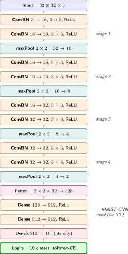
Two convolutions lift the 1-channel grayscale input to 32 channels, maxPool halves the spatial resolution, then the flattened \(14 \times 14 \times 32 = 6272\) feature vector goes through three dense layers into 10-class logits. No batch norm yet, because BN shows up in Chapter 4.

Code: the full training program

Same format as the MLP chapter. The only thing that changes from Chapter 2’s training program is the layers list. This is the spec §3.1 actually ran.

-- 1
import LeanMlir.Verified.NetsCore
import LeanMlir.Verified.Train

-- 2
def cnnVerified : VerifiedNetSpec where
  name     := "MNIST-CNN"
  slug     := "cnn"
  inC      := 1
  imageH   := 28
  imageW   := 28
  data     := .mnist
  layers   := [.conv 1 32 3 1, .relu, .conv 32 32 3 1, .relu, .maxPool 2 2,
               .flatten,
               .dense 6272 512, .relu, .dense 512 512, .relu, .dense 512 10]
  blurb    := "MNIST-CNN via the VERIFIED renderer
                (conv→conv→pool→512→512→10) → %LOWERER% → GPU"
  lossSlot := true

-- 3
def cnnConfig : VerifiedConfig where
  epochs    := 12
  batchSize := 128

-- 4
def main (argv : List String) : IO Unit :=
  cnnVerified.toNet.train cnnConfig (argv.head?.getD "data")

Walking through the numbered sections:

1. The import. Same as Chapter 2.

2. The architecture. Eleven entries: two .conv layers at 32 channels, a .maxPool, a .flatten, three .dense layers down to 10, and four .relus between them. .conv ic oc k stride takes in-channels, out-channels, kernel size and stride — no activation argument, because activations are their own entries here rather than a field on the layer that precedes them. That is why Chapter 2’s five-entry list became eleven and not seven.

The .conv2d backward pass is the theorem from earlier in this chapter (Theorem 34): the input VJP is another convolution, using the kernel reversed along both spatial axes. The max-pool backward (Definition 38) routes the gradient to the argmax position in each \(2 \times 2\) window. The dense backward is Theorem 18. Adding convolution to the model introduces no new training-loop code, only new layer types, which the framework already knows how to compose.

Two fields carry over from Chapter 2 and do the same jobs: blurb is the banner the run prints, and lossSlot declares that this render returns a trailing report-only %loss, which is the one line of verified_mlir/cnn_train_step.mlir that is not pretty of a proven graph node — the render labels it as such in a comment of its own. Everything else in the file is: Proofs.StableHLO.cnnTrainStepText emits it, and CnnFold proves that each of the ten parameter updates denotes the certified softmax cross-entropy loss-descent step derived from the Mathlib \(\operatorname {fderiv}\) math. Both convolutions, the max pool, the three dense layers and the SGD update are proof-backed operations.

3. The training hyperparameters. Twelve epochs at batch 128, SGD, no regularization and no augmentation. Note what a VerifiedConfig does not carry: the learning rate. It is baked into verified_mlir/cnn_train_step.mlir, which is §1.6’s point in a second chapter — the rate is inside the reach of the proofs, so it cannot be set to one thing and trained at another.

4. The program entry point. One line, same as the MLP chapter. cnnVerified.toNet.train cnnConfig replaces mlpVerified.toNet.train mlpConfig. That’s the whole diff.

What .conv, .maxPool and .flatten contribute.

Three more arms on Chapter 1’s toSpecs, and only one of them carries parameters:

  | conv ic oc k _ => #[(#[oc,ic,k,k],0),(#[oc],2)]   -- W, bias
  | maxPool _ _    => #[]
  | flatten        => #[]

Pooling and flattening are pure reshapes of data, so they have nothing to initialise — which is the parameter-list statement of the same fact the backward passes above make: maxPool2’s VJP routes gradient without owning any, and flatten’s is a reshape. Fold the eleven-entry list through those arms and you get the 10 params, 3489130 floats the run printed: two conv kernels and their biases, three dense matrices and theirs.

Results

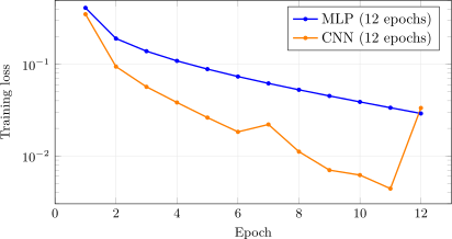
The run in §3.1 is the result. Its per-epoch training loss, against Chapter 2’s MLP on the same recipe:

MNIST, SGD 0.1, log-scale mean training loss per epoch (runs/2026-09-01-{mlp,cnn}-verified-xla-cuda/), both nets now on the same twelve. The CNN sits below the MLP through epoch 11 and reaches by epoch 5 a loss the MLP has not reached by twelve. Test accuracy is 98.77% against the MLP’s 97.81%.

The exception is the last point, and it is the interesting one. The CNN’s training loss bumps at epoch 7 and then jumps almost eightfold at epoch 12, from \(0.0044\) to \(0.0334\) — far enough to cross back above the MLP’s \(0.0291\). That is ordinary SGD at \(\text{lr}=0.1\) rather than a measurement artifact. And the run’s test accuracy is at its highest on that same epoch, 98.77%. Training loss and held-out accuracy are different measurements, and a figure where the two disagree this loudly is the one to remember when a later chapter asks you to read a loss curve.

Both curves come off the binaries these chapters’ theorems describe.

Why this network is still 99% dense-head

At 3,489,130 total parameters, the no-BN CNN is actually \(\sim \)5.2\(\times \) bigger than the MLP, not smaller. You might have expected the opposite, because convolutions are supposed to be parameter-efficient. They are, but the head is what’s eating the budget: the flatten of a \(14 \times 14 \times 32\) feature map produces a 6272-dim vector, and the first dense layer (6272 \(\to \) 512) alone is 3,211,776 parameters. The entire conv+maxPool backbone is 9,568 parameters, which is 0.27% of the total.

This is the same “fat FC head” pattern you’ll see in AlexNet, VGG, and YOLOv1: a compact convolutional backbone spending its parameter budget on a large fully-connected classifier. ResNet (Chapter 5) is the first architecture in this book without one: its head is a globalAvgPool followed by a single small dense layer, which is why ResNet-18 (a smaller version of ResNet-34) has \(\sim \)11M parameters for 1000-class ImageNet but Chapter 3’s 10-class MNIST CNN has 3.5M.

The fat head is fat because it can be, not because it must be

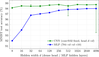
If the dense head holds 99% of the parameters, the obvious question is how many of them earn their keep. The parametric renderer answers it directly: mnist-cnn-grid holds the convolutional backbone fixed at 32 channels and sweeps only the dense head (\(\ldots {\to }d{\to }d{\to }10\)), rendering each width from the faithful CNN emitter. Overlaying that sweep on the MLP’s (both trained on their own verified StableHLO) shows how little the head needs once good convolutional features exist:

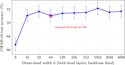
Classifier-head width sweep for the verified CNN (convolutional backbone held at 32 channels), overlaid on the MLP width sweep of Chapter 2 (runs/cnn_grid_rep{1..5}.tsv and runs/mlp_grid_results_xla.tsv). Each CNN point is the median of five runs and its whiskers are the observed range across those five — not an interval, just the highest and lowest the configuration actually produced. Eight of the ten widths repeat to within 0.4 and their whiskers are barely visible. The other two do not: \(d=512\) dropped one run to 96.66% and \(d=4096\) one to 93.52%, which is what the two long tails are.

Those tails are the reason this curve is a median of five. A symmetric error bar would have been the wrong shape for them — four runs cluster and one falls away, so there is no spread to put a \(\pm \) on — and the 95% interval on the test set, \(\pm 0.22\) at this accuracy, would have hidden a five-point failure behind a rounding error. The MLP points are single runs, which Chapter 2 reads with half a point of give.

The cost is that a handful of runs cannot see this. Draw five of the thirty runs in §3.1, build the ordinary 95% interval on their mean, and ask whether it contains the mean of the twenty-five you did not draw: it does 79% of the time, not 95%, because five draws usually miss the tail and report a spread as small as \(0.05\) against the true \(0.27\). Chapter 2’s MLP, whose thirty runs are unremarkable, gets 92% from the same procedure. How many runs a claim needs is a property of the network, and a convolution’s is higher than a dense stack’s. The early epochs of a conv net are not a measurement; the last one is, and even then not from a single run.

The whole CNN curve sits about a point above the MLP’s, and it is flat across the entire range: an 8-wide head already reaches 98.2% at 60K parameters, beating the widest 4096-wide MLP. So the 3.2M-parameter \(6272{\to }512\) layer is not buying accuracy, because shrinking the head to \(\ldots {\to }8{\to }8{\to }10\) keeps essentially all of it. The head is fat because the flatten hands it a 6272-vector and nobody trimmed it, not because the task needs the width.

3.4 MLIR: Convolution

What is already proven. mnistCnnNoBnForward is the conv \(\to \) relu \(\to \) conv \(\to \) relu \(\to \) maxPool \(\to \) flatten \(\to \) dense network, and mnistCnnNoBnHasVJPAt (Theorem 39) proves its reverse-mode derivative by chaining the per-layer VJPs: the dense backward (Theorem 18), the max-pool backward (maxPool2HasVJP3, Definition 38), and the convolution backward (conv2dHasVJP3, Theorem 34), all through the IR-level chain rule vjpCompAt. The convolution’s reverse-mode derivative is the chapter’s headline result: the input VJP of a conv2d is another conv2d, against the kernel with its in- and out-channels swapped and both spatial axes reversed. The parameter gradients are pinned by conv2dWeightGradHasVJP (the transpose trick) and the dense grads (Theorems 19, 20), and the loss gradient by softmaxCE_grad (Theorem 21). So what the convolution’s gradient is, is not in question.

The gap and how we close it. The emitted backward convolution is given a denotation \([\! [\cdot ]\! ]\) valued in the proofs’ own tensor type,

where \(\bar k = K - 1 - k\) is the spatial flip, and the bridge theorem

says the denotation of that graph is the proven conv input-VJP, the reversed-kernel identity that mnistCnnNoBnHasVJPAt only asserts. It is discharged here by expansion at the concrete shape (and again at the \(2{\to }2\) shape, by conv_back_bridge_2to2). The printer walks the graph and emits one stablehlo op per node: transpose for the channel swap, reverse for the spatial flip, convolution for the contraction. Here it is for the first conv’s backward (\(1{\to }2\) channels, \(3\times 3\) kernel, at \(4\times 4\)):

func.func @conv_back(%dy: tensor<1x2x4x4xf32>,
    %W: tensor<2x1x3x3xf32>) -> tensor<1x1x4x4xf32> {
  %Wt = stablehlo.transpose %W, dims = [1, 0, 2, 3]
          : (tensor<2x1x3x3xf32>) -> tensor<1x2x3x3xf32>
  %Wr = stablehlo.reverse %Wt, dims = [2, 3] : tensor<1x2x3x3xf32>
  %dx = stablehlo.convolution(%dy, %Wr)
      dim_numbers = [b, f, 0, 1]x[o, i, 0, 1]->[b, f, 0, 1],
      window = {stride = [1, 1], pad = [[1, 1], [1, 1]],
                lhs_dilate = [1, 1], rhs_dilate = [1, 1]}
      : (tensor<1x2x4x4xf32>, tensor<1x2x3x3xf32>)
          -> tensor<1x1x4x4xf32>
  return %dx : tensor<1x1x4x4xf32>
}

Read it against the graph: %Wt is the transpose dims [1,0,2,3] that swaps the kernel’s out- and in-channel axes, and %Wr is the reverse dims [2,3] that flips both spatial axes (\(\bar k_h,\bar k_w\)). Together they build reverseSwap \(W\). The convolution then convolves the incoming cotangent %dy against that kernel, exactly \(\texttt{conv2d}\, (\texttt{reverseSwap}\, W)\), the \(1\, \text{channel} \leftarrow 2\, \text{channels}\) adjoint of the forward conv. The bridge theorem is precisely the claim that this text computes conv2dHasVJP3’s backward. The max-pool, flatten, dense, and relu nodes of the full backward are bridged the same way, and the max-pool select_and_scatter by maxpool_back_bridge, the dense dot_generals exactly as in Chapter 2, so the whole CNN backward is covered, op by op.

Caveats.

• The convolution bridge is unconditional. A convolution is linear, so it holds at every input.

• ReLU is a smooth-point bridge (no pre-activation exactly zero), failing only on that measure-zero set.

• Max-pool is a smooth-point bridge too. It holds where every \(2\times 2\) window attains its maximum at one cell (MaxPool2Smooth); the other cells may tie with each other. An all-zero post-ReLU window fails it, so for pooling the excluded set is not measure-zero the way ReLU’s kink is, and the whole-net theorem states it as a hypothesis (h_mp in Theorem 39).

• Representative scale. \(1{\to }2\) channels at \(4\times 4\) (production: \(1{\to }32\) at \(28\times 28\)).