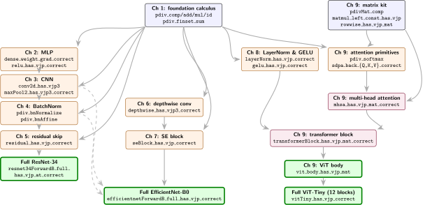
8 ConvNeXt

ConvNets strike back

By 2022 the conventional read on image recognition had flipped. ResNet had been the default backbone for six years. Then in late 2020 ViT (Dosovitskiy et al., arXiv:2010.11929) showed that a pure transformer could match or beat ResNet on ImageNet at sufficient scale, and a year later Swin (Liu et al. 2021, arXiv:2103.14030) layered in hierarchical attention to win COCO/ADE20K on top of that. The research community’s working assumption became “transformers beat convnets for vision now.”

ConvNeXt (Liu et al. 2022, arXiv:2201.03545) was a deliberate stress test of that assumption. The authors started from a standard ResNet-50 and asked: which of the design differences between ResNet and Swin is actually doing the work? They proceeded by applying transformer-era choices to the ResNet one at a time and measuring each contribution in isolation. The full list:

1. Training recipe modernization (300 epochs, AdamW, RandAug, Mixup, CutMix, label smoothing, stochastic depth, layer scale)

2. Stage compute ratio change (from (3, 4, 6, 3) to (3, 3, 9, 3), matching Swin)

3. “Patchify” stem (replace the 7\(\times \)7 stride-2 conv with a 4\(\times \)4 stride-4 conv, matching ViT’s patch embedding)

4. Depthwise convolutions (split spatial and channel mixing, as in MobileNetV2)

5. Inverted bottleneck (1\(\times \)1 expand 4\(\times \), depthwise, 1\(\times \)1 project, MobileNetV2-style)

6. Larger kernel (depthwise 7\(\times \)7 instead of 3\(\times \)3, to approximate Swin’s window attention receptive field)

7. Fewer activations and norms (one per block instead of one per layer, again matching transformer blocks)

8. LayerNorm instead of BatchNorm

9. GELU instead of ReLU

The result: a model that’s pure convolution top to bottom, doesn’t contain a single attention operation, and matches or beats Swin-T on ImageNet at the same compute budget. The conclusion of the paper isn’t “convolutions are back.” It’s “the architectural gap between ResNet and Swin was mostly the training recipe, not the receptive field.” Most of what looked like transformer superiority was modernization that hadn’t been back-ported to the convnet baseline.

8.1 Run it first

Before the two new primitives, train the network that needs them. Four commands, and the heaviest per-epoch net in the book still finishes inside an hour and a quarter:

lake exe cache get                            # Mathlib oleans, ~30 s
./scripts/datasets/download_imagenette.sh     # 330 MB dl, 2.4 GB unpacked
lake build convnext-verified-adam
./.lake/build/bin/convnext-verified-adam data

On one RTX 4060 Ti (CUDA 12.9), from runs/2026-09-13-convnext-imagenette-ls1e-6-resident/. XLA’s startup banner and the resident-parameter notices are removed, the network description line is wrapped and its trailing LayerNorm note dropped, each interval is wrapped onto an indented continuation, and epochs 5 through 78 are elided:

[pjrt_ffi] XLA backend: PJRT 0.114, 1 device(s)
[pjrt_ffi] command buffers: enabled (CUDA default)
[pjrt_ffi] compiled verified_mlir/convnext_adam_train_step.mlir
             (@convnext_adam_train_step, 549 outputs, 1 replica)
             in 6361 ms
[pjrt_ffi] compiled verified_mlir/convnext_fwd.mlir
             (@convnext_fwd, 1 outputs, 1 replica) in 588 ms
ConvNeXt-T on Imagenette 224² (patchify /4 → stem channel-LN →
  [3,3,9,3] blocks @ [96,192,384,768] depthwise-7×7 + channel-LN +
  GELU + layerScale + 3 downsamples 56→7 → GAP → LN → dense)
  via the VERIFIED renderer → XLA/PJRT → GPU
  xla/pjrt verified_mlir/convnext_adam_train_step.mlir
  xla/pjrt verified_mlir/convnext_fwd.mlir
  train 9469, val 3925; bs 32, ConvNeXt-T adam
    (cosine+warmup 3ep, baseLR 0.001000), He init
Epoch 1/80: loss=2.321469 lr=0.000333
  epoch 1: val_acc = 1106/3925 = 28.178344%  top5 = 2873/3925 = 73.197452%
    [95% CI 26.79–29.61]
Epoch 2/80: loss=2.000190 lr=0.000667
  epoch 2: val_acc = 1566/3925 = 39.898089%  top5 = 3378/3925 = 86.063694%
    [95% CI 38.38–41.44]
Epoch 3/80: loss=1.675131 lr=0.001000
  epoch 3: val_acc = 2057/3925 = 52.407643%  top5 = 3601/3925 = 91.745223%
    [95% CI 50.84–53.97]
Epoch 4/80: loss=1.506907 lr=0.001000
  epoch 4: val_acc = 2226/3925 = 56.713376%  top5 = 3640/3925 = 92.738854%
    [95% CI 55.16–58.26]
Epoch 79/80: loss=0.500732 lr=0.000000
  epoch 79: val_acc = 3230/3925 = 82.292994%  top5 = 3789/3925 = 96.535032%
    [95% CI 81.07–83.46]
Epoch 80/80: loss=0.500793 lr=0.000000
  epoch 80: val_acc = 3229/3925 = 82.267516%  top5 = 3788/3925 = 96.509554%
    [95% CI 81.04–83.43]
done (trained ConvNeXt-T adam + cosine/warmup via packed threading).

Eighty epochs at about 55 seconds each, one hour and fourteen minutes in total, and 82.27% top-1 with 96.51% top-5 on Imagenette’s 3,925-image validation split. The best epoch reached \(82.32\% \). That is the lowest top-1 of the convnets in this book’s Imagenette column, from much the largest network among them, and §8.3 is about why that is the expected answer rather than a defect.

Two compile lines, where the previous three chapters each had three. ResNet-34, MobileNetV2 and EfficientNet-B0 all emit a third artifact, <slug>_fwd_eval, because BatchNorm behaves differently in training and in evaluation and the evaluation forward has to read frozen running statistics. ConvNeXt has no BatchNorm. LayerNorm computes its statistics from the activation in front of it every time, so there is nothing to freeze, and the training forward and the evaluation forward are the same function. The chapter’s central swap pays for itself in the build before it pays for itself in the mathematics.

That also shows in the first four epochs. Top-1 climbs 28.2, 39.9, 52.4, 56.7, smoothly. A BatchNorm net can show a step in its first epochs, when the running statistics average over weights that are still moving fast and the evaluation forward briefly uses statistics that no longer describe the network (Chapter 7). No such step exists here, because no such statistics exist here.

Three new operations this chapter, still three rules. What ran is pretty(provenGraph), the file verified_mlir/convnext_adam_train_step.mlir, and every channel-LayerNorm in it backpropagates by Theorem 96 (the head’s vector LayerNorm by Theorem 126), every GELU by Theorem 97, every layer scale by its own diagonal adjoint, every depthwise convolution by Theorem 71, and every residual skip by Theorem 58.

And the fold holds at full depth. convNextForwardTChHasVJP chains the patchify stem, all eighteen ConvNeXt blocks, the three downsamples, the pool and the head through vjpComp, with convNextForwardTChHasVJP_correct carrying it back to the forward the spec denotes. It assumes 23 positive LayerNorm epsilons and nothing else. Unlike Chapter 6, whose full-depth fold is pointwise because relu6’s kink makes a statement over all inputs false, this one is a single global HasVJP over the entire network, and it can be because GELU is smooth everywhere. So for ConvNeXt the accurate sentence is the strong one: every operation in the graph that just trained carries a proved backward, and their composition into the whole network carries one too.

Two new primitives

ConvNeXt requires two activations / normalizations that the chapters so far haven’t needed:

LayerNorm (Ba, Kiros, Hinton 2016, arXiv:1607.06450). BatchNorm normalizes per-feature across a batch: it relies on the batch having enough samples for the mean and variance to be stable. That fails for small batches (memory-constrained training) and for variable-length sequences (where “the batch axis” isn’t a clean concept). LayerNorm solves both by flipping the axis: normalize per-sample across the feature dimension instead. Same three-term Jacobian cancellation as BN (Chapter 4), same closed-form backward. Just a different reduction axis. Theorem 95 states this formally for one vector, and Theorem 96 lifts it to the channel axis of a feature map.

GELU (Hendrycks & Gimpel 2016, arXiv:1606.08415). A smooth approximation of ReLU: \(\mathrm{GELU}(x) = x \cdot \Phi (x)\), where \(\Phi \) is the standard-normal CDF. ReLU has a kink at zero, which forces the codegen to substitute a subgradient convention (Chapter 2). GELU is differentiable everywhere, with a soft-gate behavior near zero that empirically helps transformers (and, it turns out, modernized CNNs). Diagonal activation Jacobian, same family as ReLU’s diagonal, just with a smooth scalar derivative instead of an indicator. Theorems 92–97 provide the scalar function, its derivative, the Jacobian, and the assembled VJP.

Both primitives are used by the upcoming Vision Transformer chapter (Chapter 9) without modification. ConvNeXt introduces them here so they’re available before ViT needs them.

The ConvNeXt block

Each ConvNeXt block stacks the modernization items into a single residual unit:

Two pieces: the inverted bottleneck (\(1 \times 1\) expand 4\(\times \), depthwise spatial conv at the wide point, \(1 \times 1\) project) is exactly the MobileNetV2 inverted residual from Chapter 6. ConvNeXt is paying the MobileNet idea forward. LayerScale (Touvron et al. 2021) is a learnable per-channel scalar \(\gamma \) initialized to \(10^{-6}\) that multiplies the block’s contribution before the residual add, keeping the block near-identity at init in the same spirit as ResNet’s residual. The spec’s .convNextStage primitive emits \(N\) of these blocks at fixed channel width. The .convNextDownsample primitive emits the LN + \(2 \times 2\) stride-2 conv that transitions between stages.

ConvNeXt-T is four stages, ResNet-style

The full ConvNeXt-T spec is the same stem–stages–head template as ResNet-34. A \(4 \times 4\) stride-4 “patchify” stem replaces the \(7 \times 7\) stride-2 stem. Four stages with block counts \((3, 3, 9, 3)\) at channel widths \((96, 192, 384, 768)\) replace the ResNet stages. A final global-average-pool plus 768-to-10 dense replaces the head. Total: 27.8M parameters, comparable to ResNet-50. Every architectural primitive in the spec is now codegen-backed and has a proved VJP. None of the math in this chapter is genuinely new beyond the LayerNorm-axis rotation and the GELU smoothness.

With a modernized convnet backbone, the dominant axis of variation between runs becomes the training recipe, not the architecture. The example section below makes that concrete. The chapter closes by putting the full recipe side-by-side with the 2018 ResNet-34 recipe of Chapter 5, knob by knob: the four-year jump in how convnets are trained, on one page.

8.2 The theorems

Three rungs of the ladder for ConvNeXt-T: the rendered backward is the VJP, with the whole-net VJP folded into it; the emitted step is the certified step; each node is the loss’s derivative.

8.3 Example: ConvNeXt-T on Imagenette

The architecture

ConvNeXt-Tiny replaces the convolutional stages with .convNextStage blocks at four widths (\(96, 192, 384, 768\)) and depths (\(3, 3, 9, 3\)), glued by .convNextDownsample transitions (LayerNorm \(+\) \(2 \times 2\) stride-2 conv). A \(4 \times 4\) stride-4 patchify stem and a global-average-pool head bracket the stack. The inset shows one ConvNeXt block: an inverted bottleneck with a single LayerNorm and GELU, scaled by a learnable \(\gamma \) before the residual add.

The verified trainer

The pattern is §5.3’s, minus bnChannels: there is no BatchNorm.

import LeanMlir.Verified.NetsCore
import LeanMlir.Verified.Train

-- 1. The network. `slug` names the committed render. No `bnChannels`:
--    LayerNorm keeps no running statistics, so nothing has to be
--    threaded from training into evaluation.
def convnextVerified : VerifiedNetSpec where
  name     := "ConvNeXt-T"
  slug     := "convnext"
  inC      := 3
  imageH   := 224
  imageW   := 224
  data     := .imagenette
  layers   := [
    .conv 3 96 4 4, .layerNorm 96,       -- patchify 4x4/s4 + stem LN
    .convNextBlockCh 96,  .convNextBlockCh 96,  .convNextBlockCh 96,
    .layerNorm 96,  .conv 96 192 2 2,    -- downsample  96->192, 56->28
    .convNextBlockCh 192, .convNextBlockCh 192, .convNextBlockCh 192,
    .layerNorm 192, .conv 192 384 2 2,   -- downsample 192->384, 28->14
    .convNextBlockCh 384, .convNextBlockCh 384, .convNextBlockCh 384,
    .convNextBlockCh 384, .convNextBlockCh 384, .convNextBlockCh 384,
    .convNextBlockCh 384, .convNextBlockCh 384, .convNextBlockCh 384,
    .layerNorm 384, .conv 384 768 2 2,   -- downsample 384->768, 14->7
    .convNextBlockCh 768, .convNextBlockCh 768, .convNextBlockCh 768,
    .globalAvgPool, .layerNorm 768, .dense 768 10 ]   -- head: GAP -> LN -> dense
  -- Stochastic depth, read only by the `*drop` variants: one global
  -- block index over the eighteen blocks, keep_i = 1 - 0.1*i/17.
  dropSites := Array.range 18
  dropDenom := 17
  dropRate  := 0.1
-- 2. The schedule. ResNet-34's, MobileNetV2's and B0's, unchanged.
def convnextAdamConfig : VerifiedConfig where
  epochs    := 80
  batchSize := 32
-- 3. The entry point: AdamW, cosine with a 3-epoch warmup, baseLR 1e-3.
--    The EMA decay and the drop rate are env knobs.
def runConvNeXtAdam (argv : List String) : IO Unit := do
  let variant := (← IO.getEnv "LEAN_MLIR_VARIANT").getD "adam"
  let emaDecay := match (← IO.getEnv "LEAN_MLIR_EMA_DECAY_U").bind (·.toNat?) with
    | some u => u.toFloat * 1e-6
    | none   => 0.9999
  let dropNet := match (← IO.getEnv "LEAN_MLIR_DROP_RATE_U").bind (·.toNat?) with
    | some u => { convnextVerified.toNet with
                  dropKeeps := convnextVerified.dropKeepsAt (u.toFloat * 1e-6) }
    | none   => convnextVerified.toNet
  dropNet.trainAdamSched convnextAdamConfig
    (argv.head?.getD "data") 0.001 0.9 0.999 3 variant 0.0 1.0 emaDecay
def main (argv : List String) : IO Unit := runConvNeXtAdam argv

The structure follows the paper’s macro-design prescription: 4 stages with block counts \((3, 3, 9, 3)\) and channels doubling on every downsample \((96 \to 192 \to 384 \to 768)\), with the heavy 9-block stage at the \(14 \times 14\) / 384-channel resolution. The stem is a \(4 \times 4\) stride-4 conv (mirrored from ViT’s patch-embed), not the \(7 \times 7\) stride-2 stem of a ResNet, and that is one of the nine modernization items listed at the top of the chapter. The base recipe — AdamW at \(10^{-3}\), cosine with a three-epoch warmup, weight decay \(10^{-4}\), label smoothing \(0.1\) — is Chapter 5’s (§5.6 measures each knob), so the comparison across architectures is of the architecture.

.convNextBlockCh c is one block per line, eighteen of them. Ch names the norm: the LayerNorm inside the block reduces over the c channels at each spatial position, which is ConvNeXt’s real normalization rather than the scalar reduction the bare name suggests.

The arm, and the one tensor with no partner.

  | layerNorm d      => #[(#[d],1),(#[d],2)]           -- Ch. 8: gamma, beta
  | convNextBlockCh c =>                               -- Ch. 8
    #[(#[c,1,7,7],0),(#[c],2),(#[c],1),(#[c],2),       -- dw 7x7 + LN(gamma,beta)
      (#[4*c,c,1,1],0),(#[4*c],2),                     -- expand 1x1 (4x)
      (#[c,4*c,1,1],0),(#[c],2),                       -- project 1x1
      (#[c],3)]                                        -- layer scale, init 1e-6

Eight of those nine tensors pair off into weight-and-bias or \(\gamma \)-and-\(\beta \). The ninth, the trailing (#[c],3), has no partner: layer scale is a single learned per-channel multiplier with nothing added after it, and kind 3 is its own initialiser, the paper’s \(10^{-6}\), so a fresh block starts near the identity on its residual branch. It is the smallest parameter in the chapter and the one whose backward is a pure diagonal.

The wrong init is worth three points here. Until 2026-09-13 the verified path initialised layer scale to ones, and the same render on the same recipe landed at \(85.45\% \) against the \(82.27\% \) above, resolved at \(\pm 1.2\) per run (runs/2026-08-30-convnext-imagenette-headln/). The two are level through epoch 10 and three to four points apart from epoch 20 on (\(80.87\) against \(77.43\) at 20, \(84.18\) against \(80.03\) at 40): with \(\gamma \) at \(10^{-6}\) every residual branch’s gradient is scaled by \(\gamma \), so the branches train late, and 9,469 images over 80 epochs never make the time up. The recipe this init belongs to is 300 epochs on 1.28M images, where a late start costs nothing, and §8.5 is that regime. The book keeps the paper’s value because it is the paper’s and the JAX reference’s; the ones run is the better number on this recipe and not the paper’s initialisation.

The stem and the downsamples are spelled out, not packaged. A .convNextDownsample 96 192 is two entries here, a .layerNorm 96 and a .conv 96 192 2 2, and the patchify stem is likewise a .conv followed by a .layerNorm. The spec’s job is the parameter layout, not the block vocabulary, so it names weights rather than concepts.

182 parameter tensors, 27,827,818 scalars. convnextVerified.toSpecs is kernel-#guarded against ConvNeXtLayout.specs, an independently audited hand-list, and the ImageNet spec of §8.5 is pinned to this one at everything but its head. At 1000 classes the count is 28,589,128, which is timm’s figure for convnext_tiny exactly.

Twenty-three LayerNorms are the entire hypothesis budget. One in the stem, one per block, one per downsample, and one on the head between the pool and the classifier. Theorems 96 and 126 want \(\varepsilon {\gt} 0\) at each, and those 23 positivities are the only assumptions anywhere in the chain.

Results

§8.1 has the run: 80 epochs at about 55 seconds each, one hour and fourteen minutes, \(\mathbf{82.27\% }\) top-1 and \(\mathbf{96.51\% }\) top-5, with the loss settling on the same \({\sim }0.50\) label-smoothing floor as the three chapters before it. The four-chapter comparison — same dataset, same recipe, same eighty epochs, and every row a measurement on the verified XLA path, on one RTX 4060 Ti:

Columns as in Chapter 7’s table; ResNet-34’s row is the five-seed mean of §5.6 (runs/2026-09-12-r34-ablation-fp32-seeds/) with one seed’s timing.

• The largest convnet in the column finishes last among them, and by a clear margin: \(82.27\% \) against \(89.99 \pm 0.32\) for ResNet-34 and \(90.04\% \) for EfficientNet-B0, from \(1.3\times \) and \(6.9\times \) their parameters. Three things contribute. ConvNeXt-T carries 27.83M parameters against 9,469 training images, which is not the data scale that capacity wants. The recipe here is the shared one, AdamW at \(10^{-3}\) with cosine and label smoothing, which is deliberately not the recipe ConvNeXt was designed around. And its layer scale starts at the paper’s \(10^{-6}\), which on this short schedule is worth three points on its own (above).

• That is the chapter’s thesis arriving as a result rather than a claim. ConvNeXt’s paper argues the modernization lives in the training recipe, so a ConvNeXt run on somebody else’s recipe should underperform, and it does. §8.5 is the control: the same architecture, given the full DeiT pack and 300 epochs, reaches \(81.53\% \) on ImageNet-1k and beats every other network in this book. The architecture was never the variable.

• It is the slowest per step, at 188 ms against ResNet-34’s 120 and EfficientNet-B0’s 103. The depthwise \(7 \times 7\) and the channel LayerNorms touch every spatial position twice per block, and the \(4\times \) expansion makes its \(1 \times 1\)s the largest matmuls in the column.

• The MLIR is mid-pack at 1,019 KB, above ResNet-34’s 754 and below MobileNetV2’s 1,047 and EfficientNet-B0’s 1,316. Block count is not what separates them, since ConvNeXt’s eighteen is more than either. What separates them is what one block costs to emit: ConvNeXt spends three convolutions and a single LayerNorm per block, while an inverted residual spends three convolutions and three BatchNorms, and an MBConv adds the squeeze-excitation pair on top of that. One normalization per block instead of one per layer was item seven on the modernization list, and it is visible in the file size.

8.4 MLIR: Layer Scale

Layer scale is a per-channel learnable diagonal, \(\mathrm{layerScale}(\gamma , x) = \gamma \odot x\), and it is the simplest operator in this series. Its Jacobian is diagonal, so it is its own adjoint: layerScaleHasVJP proves \(\mathrm{back}(x, dy) = \gamma \odot dy\), the backward multiplying by the same \(\gamma \) the forward did. There is nothing to bridge past that identity, so the emitted graph is two multiplys against one tensor:

// ConvNeXt block tail:  out = x + layerScale(gamma, project(...))
%ls  = stablehlo.multiply %gls, %pr   : tensor<1x2x4x4xf32> // gamma (*) pr
%out = stablehlo.add %x, %ls          : tensor<1x2x4x4xf32> // + identity skip
// backward, cotangent %dOut:  d(pr) = gamma (*) d(out)
%dpr = stablehlo.multiply %gls, %dOut : tensor<1x2x4x4xf32>

The forward multiply %gls, %pr and the backward multiply %gls, %dOut are the same op against the same \(\gamma \) tensor: a diagonal map is its own transpose, so its VJP is itself. The identity skip is the residual fan-in (Theorem 58). The surrounding GELU, LayerNorm, and convolution backwards reuse their bridges. Every one is unconditional (the only hypothesis anywhere is LayerNorm’s \(\epsilon {\gt} 0\)): ConvNeXt has no kinked operator, and neither do EfficientNet-B0 and the Vision Transformer, the two other chapter nets whose whole-network VJP needs only \(\epsilon {\gt} 0\). The full block is \(\mathrm{residual}(\mathrm{layerScale} \circ \mathrm{project} \circ \mathrm{gelu} \circ \mathrm{expand} \circ \mathrm{LN} \circ \mathrm{depthwise})\), composed by convNextBlockHasVJP.

8.5 ImageNet recipe

ConvNeXt’s architecture reached this book through the Imagenette example earlier in this chapter, and the recipe runs on both paths — the reference first, then the verified path, then the two side by side.

The reference (JAX)

The reference port wires the two ConvNeXt-specific layers (.convNextStage, .convNextDownsample) into the JAX codegen. Because that path differentiates with jax.value_and_grad, only the forward had to be written, and the backward comes for free. The spec mirrors jax/MainConvNeXtImagenet.lean, its recipe quoted as the run below trained it (the file today carries the official rows, the marker’s, for the rerun):

-- Faithful patchify stem, stage/downsample backbone, 1000 classes.
def convNeXtTinyImagenet : NetSpec where
  name   := "ConvNeXt-T (ImageNet, bf16)"
  imageH := 224
  imageW := 224
  layers := [
    .convNextStem 3 96 4,              -- patchify: 4x4 s4 conv -> channel-LN (no BN/ReLU)
    .convNextStage 96 3 .ln .gelu,     -- stage 1: 3 blocks @ 96  (56x56)
    .convNextDownsample 96 192,        -- 56 -> 28
    .convNextStage 192 3 .ln .gelu,    -- stage 2: 3 blocks @ 192
    .convNextDownsample 192 384,       -- 28 -> 14
    .convNextStage 384 9 .ln .gelu,    -- stage 3: 9 blocks @ 384
    .convNextDownsample 384 768,       -- 14 -> 7
    .convNextStage 768 3 .ln .gelu,    -- stage 4: 3 blocks @ 768
    .globalAvgPool,
    .layerNorm 768,                    -- head LN: the paper's GAP -> LN -> Linear
    .dense 768 1000 .identity          -- 1000-class head
  ]

-- ConvNeXt needs AdamW, not SGD; full DeiT-style recipe.
def convNeXtTinyImagenetConfig : TrainConfig where
  learningRate      := 2.5e-4       -- 4e-3 @ batch 4096, linearly scaled to 256
  batchSize         := 256
  epochs            := 80           -- validation tier of an 80->300 ladder
  optimizer         := .adam        -- AdamW (decoupled weight decay)
  weightDecay       := 0.05
  wdExcludeNormBias := true         -- timm no_weight_decay: skip norm g/b, bias, LayerScale
  cnxInit           := true         -- ConvNeXt _init_weights: trunc_normal(0.02) on every conv
  cosineDecay       := true
  warmupEpochs      := 20           -- ConvNeXt paper warmup (was 5)
  gradClipNorm      := 1.0          -- ours: the paper does not clip
  augment           := true
  useRandAugment    := true         -- geometric RandAugment N=2, M=9, mstd0.5, inc1
  randAugmentGeometric := true
  augBicubic        := true         -- PIL-bicubic geometry, as timm (after the run below)
  randAugmentMstd   := 0.5
  randAugmentInc    := true
  useMixup          := true         -- Mixup alpha 0.8 ...
  useCutmix         := true         -- ... + CutMix alpha 1.0 (alternates per step) ...
  randomErasing     := true         -- ... + Random Erasing p 0.25 (full DeiT pack)
  randomErasingProb := 0.25
  erasingPixel      := true         -- timm mode='pixel', N(0,1) fill (after the run below)
  labelSmoothing    := 0.1
  bf16              := true
  bf16Conv          := true         -- dw-7x7 + 1x1s; LN/GELU stay fp32
  f32StemHead       := true         -- classifier head in fp32
  useEMA            := true         -- weight averaging, decay 0.9999
  dropPath          := 0.1          -- stochastic depth (ConvNeXt-T paper value)

-- 300-epoch "full" tier: same config, longer schedule.
def convNeXtTinyImagenetConfigFull : TrainConfig :=
  { convNeXtTinyImagenetConfig with epochs := 300 }

Unlike MobileNet and EfficientNet, ConvNeXt trains with AdamW and a small decoupled weight decay, not SGD. The modernized-convnet recipe is the architecture’s whole thesis. bf16Conv pays off especially here: the \(7\times 7\) depthwise is \(\sim 2.3\times \) faster in bfloat16 (a large kernel has enough arithmetic for the tensor cores to bite, unlike the \(3\times 3\) depthwise, which is a wash), and the inverted-bottleneck \(1\times 1\)s are matmuls that love it. The channel LayerNorm and GELU stay in fp32.

The elements of the paper recipe, wired and on:

• the faithful patchify stem (.convNextStem: \(4\times 4\) stride-4 conv \(\to \) channel-LayerNorm, no BN/ReLU)

• stochastic depth (drop-path 0.1) and EMA (decay 0.9999), together \({{\lt}}5\% \) per epoch

• decoupled weight decay that excludes the norm/bias/LayerScale 1-D params (wdExcludeNormBias, timm’s no_weight_decay)

• the full DeiT-style augmentation pack: Mixup \(\alpha 0.8\), CutMix \(\alpha 1.0\), Random Erasing \(p0.25\), and geometric RandAugment (\(N{=}2\), \(M{=}9\), mstd0.5-inc1)

The peak LR is \(2.5\mathrm{e}{-}4\) (the \(4\mathrm{e}{-}3\)@4096 official value linearly scaled to batch 256) over a 20-epoch warmup. No deviation from the paper’s architecture remains but the GELU, which is the tanh approximation on both paths (Definition 92); where the recipe departs from the paper’s is the marker after the side-by-side table. The run below is the full 300-epoch tier, trained and evaluated on an antialiased bicubic resize and scored at the paper’s protocol, \(224\) with a \(0.875\) centre crop.

Both figures are the exponential moving average of the weights, scored over all \(50{,}000\) validation images. The raw weights score \(81.51\% \) / \(95.50\% \), so weight averaging is worth \(+0.03\) points here — the cosine schedule anneals the learning rate to zero over the final epochs, and weights that have stopped moving leave the average nothing to remove.

The full 300-epoch tier (convnext-tiny-imagenet full, convNeXtTinyImagenetConfigFull) reached \(\mathbf{81.53\% }\) top-1 and \(\mathbf{95.50\% }\) top-5 on the held-out validation pass. That is the strongest result in this book’s sweep by a wide margin, ahead of ResNet-50 RSB-A3 (\(77.75\% \)), EfficientNet-B0 (\(77.15\% \)) and ResNet-34 (\(74.14\% \)), and it lands within \(\sim \)0.6% of ConvNeXt-T’s \(82.1\% \) paper headline from a from-scratch Lean\(\to \)JAX-codegen reimplementation. Two candidate explanations for that residual can be ruled out from this run: weight averaging is measured above and accounts for none of it, and the evaluation is the paper’s own, \(224\) at a \(0.875\) crop. What is left is the recipe departures above, not the architecture and not the eval protocol.

The validation curve tells the augmentation story directly: a deliberately slow start, since Mixup and CutMix blend labels, so the net under-trains for the first \(\sim \)20 epochs, compounded by the EMA shadow lagging the live weights. Then it climbs for the rest of the schedule without an overfitting turn, which is what the heavy-regularization regime predicts and what makes the long schedule worth buying.

Learning-rate robustness. The full pack was also a test of ConvNeXt’s learning-rate robustness under AdamW, the test Chapter 7 ran on RMSProp. It is robust: at the \(2.5\mathrm{e}{-}4\) peak with global-norm gradient clipping at \(1.0\), top-1 climbed across the whole 300-epoch schedule with no erosion and no divergence, the opposite of B0’s RMSProp blow-up. AdamW’s bounded, decoupled step plus the grad-clip makes the peak LR a non-event, which is what lets the heavy augmentation run to schedule instead of destabilizing it early.

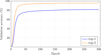
ConvNeXt-T / ImageNet-1k validation accuracy per epoch over the full 300-epoch schedule (bf16, 4\(\times \) 3060), every point the EMA weights scored over all \(50{,}000\) validation images. Neither curve turns over: both rise through the schedule and flatten across the final \(\sim \)40 epochs, where the cosine has annealed the learning rate to zero.

The verified path (PJRT)

The verified trainer trains the same network through the proof-rendered StableHLO that §8.1 ran at Imagenette scale. It is apps/imagenette/MainConvNeXtImagenet.lean, built as lake build convnext-imagenet-verified:

-- Identical backbone, 1000 classes instead of 10.
def convnextImagenetVerified : VerifiedNetSpec where
  name       := "ConvNeXt-T (ImageNet-1k)"
  slug       := "convnextin"
  data       := .imagenet
  shimScript := "generated_convnext_tiny_imagenet_shim.py"
  layers     := [ ... the Imagenette stack, 1000-class head ... ]

-- 300 epochs, because that is the schedule the reference number
-- above was measured on. Batch is 64 PER DEVICE, the reference's
-- global 256 over four replicas.
def convnextImagenetConfig : VerifiedConfig where
  epochs    := 300
  batchSize := 64
  cnxInit   := true   -- ConvNeXt _init_weights: trunc_normal(0.02), as the reference

The head is the only parameter shape that moves, from \(768 \times 10\) to \(768 \times 1000\), which takes the count from 27,827,818 to 28,589,128. Three kernel #guards hold the two specs together at everything else: equal toSpecs.size, equal toSpecs.pop.pop, and a back! of (#[1000], 2).

The collectives are gated by two gates, and they prove different things. tests/TestConvNeXtDpCheck.lean pins the data-parallel forward bit-exactly against its single-device peer. That gate hands both replicas the same rows, so it is structurally blind to a shard-offset bug, and tests/TestConvNeXtShardCheck.lean closes exactly that hole by giving the replicas genuinely different data. ConvNeXt is where the shard check was written before being generalized to the other nets, so this is the one chapter where both gates are native rather than inherited.

The regularizer knobs are render variants, and the run carries three of the four. Weight-decay exclusion, stochastic depth and this book’s gradient clip are spelled wx, drop and clip, and convnextin_adamdpwxclipdropbf16 carries all three at once on top of AdamW, bf16 and the four-way all-reduce. It is the artifact the run below used; Theorem 99 reaches its bf16 gradient nodes at its eighteen drop-path sites. EMA is rendered too, and convnextin_emadpwxclipdropbf16 carries all four, but it landed after this run, which trained adamdpwxclipdropbf16 and scores its raw weights, and the pairing below is made against the reference’s raw arm, which the reference section measured at \(0.03\) points under its EMA. Mixup and CutMix never enter the graph at all, because they are data-side and ride the shim. It runs with:

lake run cnx-default-4gpu

Global batch 256 as \(4 \times 64\) replicas at the reference’s \(2.5\mathrm{e}{-4}\) and its 5,004 steps per epoch; the raw weights at epoch 300, scored over the same \(50{,}000\) validation images. The best epoch was 291, at \(81.39\% \).

The two paths, side by side

Both columns are ConvNeXt-T on the paper’s recipe, 300 epochs, on the same four RTX 3060 cards, scored over the same \(50{,}000\) validation images. Rows above the first rule differ; rows between the rules are held equal by construction. The reference’s headline earlier is its EMA; its row here is its raw weights, because that is the arm the verified path has. [TODO: the official recipe in four places, on both paths: batch \(4096\) (accumulated \(16\times \) at \(256\), exact without BatchNorm), no gradient clip, Mixup or CutMix drawn per batch, torchvision’s crop; plus the exact erf GELU, the cosine floor at \(10^{-6}\), RandAugment’s fill at the image mean, the EMA decay constant from step \(0\), an fp32 evaluation forward, and scoring at timm’s \(288\) / \(1.0\). The EMA pair, in code since 2026-10-12, has not run; one rerun of both halves takes all of it — cnx-default-jax-4gpu / cnx-default-emabf16-4gpu, \({\sim }76 + 109\) h.]

The two paths agree to \(0.21\) points on top-1 and \(0.11\) on top-5, inside the 95% Wilson interval (\(\pm 0.34\) at \(81\% \) on \(50{,}000\) images), at one seed each. This is the chapter where the pair can say more than that, because both checkpoints were scored on the same images in the same order, so the comparison can be paired instead of read off two intervals. Of the \(50{,}000\), both paths get \(38{,}850\) right and \(7{,}445\) wrong; \(1{,}903\) are right only on the reference and \(1{,}802\) only on the verified path. McNemar’s exact test asks whether those \(3{,}705\) discordant images split unevenly, and answers \(p = 0.10\) (scripts/demos/mcnemar.py): a net of \(101\) flips does not separate the two checkpoints. The alignment was checked rather than assumed — the two agree on \(92.6\% \) of images, where unrelated orderings would agree on \(69.7\% \). What the pair does not isolate is variance. The drop-path and Mixup masks are host-drawn on one path and jax.random’s on the other, and the seeds differ, so \(7.4\% \) of images decided differently is what two ConvNeXt-Ts differing in seed and mask source disagree on here; a two-seed pair on one path, which would bound the spread alone, has not been run. “Not separable” is the claim, not “identical”. Like ViT, ConvNeXt has no BatchNorm to normalize over a different group; unlike ViT, its verified arm ran without EMA, so this is a two-variable pair with the second variable measured at \(0.03\).

The curves are read with one caveat, and it is the EMA. The reference’s per-epoch evaluation scores its EMA shadow (decay \(0.9999\), about a two-epoch time constant) and the verified path scores its raw weights, so mid-schedule the figure compares an averaged model to a live one. The figure shows it: the verified path leads from epoch 3 to 17, by up to \(2.8\) points, while the shadow lags a fast climb; it trails by up to \(4.1\) points at epoch 33, at peak learning rate, where averaging is worth the most; and the gap closes as the cosine anneals, to a mean of \(0.28\) points over the last fifty epochs. Only the final pairing above is raw against raw. A raw reference curve cannot be rebuilt after the fact — the reference kept raw weights only for its last three epochs — which is why the reference section measured the EMA’s worth at the end, where it is \(0.03\), and not along the way, where it is several points.

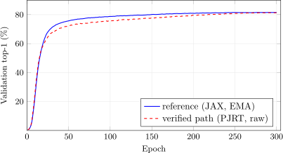
One recipe, two paths to XLA, every epoch, scored over all \(50{,}000\) validation images.

The remaining \(91.3\) against \(76.5\) hours is \(1.23\times \) per step, \(220\) against \(179\) ms at the same shape on the same cards. Of the \(41\) ms, \(15\) is the feed — the fed step against the step with the shim removed, measured on this box — which is \(6.8\% \) of the step on the heaviest shim in the book (RandAugment and random erasing per image), because doubling the per-replica batch from \(32\) to \(64\) doubled the arithmetic each augmented image amortizes over. The other \(26\) is the lowering, read against §9.6’s accounting.

What the ConvNeXt recipe changes from the 2018 recipe

The ResNet-34 trainer of Chapter 5 is the 2018-era recipe: the original paper’s SGD-with-momentum plus the “bag of tricks” polish (cosine schedule, warmup, label smoothing, random-resized-crop). The config above is the 2022 ConvNeXt recipe, DeiT’s transformer-training playbook applied to a convnet. Where Chapter 5’s RSB-A3 side quest showed the 2018\(\to \)2021 jump on a fixed ResNet, this table shows the 2018\(\to \)2022 jump with the block modernized in step. Since “the recipe is the thesis” is this architecture’s whole argument, the diff below is the chapter in table form. The trainAdamSched entry point is identical in both columns, and every row is a one-line change to the VerifiedNetSpec, the VerifiedConfig, or the arguments beside them:

What carries over unchanged: cosine LR decay, the warmup-then-anneal structure, random-resized-crop + horizontal flip as the base augmentation, label smoothing \(0.1\), batch 256 (the paper’s own batch is \(4096\), and the peak LR is scaled for it), train and eval both at \(224\) (no FixRes), and bf16 convolution under an fp32 classifier head.

The augmentation row is the full DeiT pack: Mixup (Zhang et al. 2017, arXiv:1710.09412), CutMix (Yun et al. 2019, arXiv:1905.04899), Random Erasing (Zhong et al. 2017, arXiv:1708.04896), and RandAugment (Cubuk et al. 2019, arXiv:1909.13719). All four are implemented as data-only kernels that mutate the input tensor before the graph sees it, tier 1 in our codegen scope, no MLIR plumbing required. Mixup and CutMix route through a soft-label train-step variant since they produce fractional labels. Random Erasing and RandAugment leave labels alone.

The through-line is the same “regularize harder, train bigger” as RSB-A3, arrived at from the transformer side: keep cross-entropy and soften the targets instead of switching losses, AdamW instead of LAMB (the batch stays moderate), stochastic depth and EMA from the ViT toolkit, and a \(3\times \) longer schedule to let the regularization pay.

8.6 Side quest: scaling to ConvNeXt-S and B

The axis. Scaling ConvNeXt-T is two moves. S deepens stage 3 from 9 blocks to 27 and touches nothing else; B does that and widens every stage, \(96/192/384/768 \to 128/256/512/1024\). On the JAX side both are parameter edits. On the verified side they are not the same job at all.

Every number in this section was measured on 4\(\times \) RTX 4060 Ti (16 GB, CUDA 12.9). Counts are #guarded at \(50{,}223{,}688\) and \(88{,}591{,}464\), \(344\) tensors each, the head LayerNorm’s \(\gamma \) and \(\beta \) included.

A full schedule, four cards, \(300\) epochs at the jobs’ own shape — \(64\) per replica, sixteen micro-batches accumulated to the official \(4096\), \(312\) updates an epoch — with each path’s own trainer timed on real ImageNet (the 2026-10-12 smokes):

Totals include the per-epoch evaluation; the verified steps are fed, \(3\)–\(7\) ms of them waiting on the shim. All four are compute-bound.

What is queued. Both pairs exist. The verified jobs are cnx{s,b}-default-emabf16-4gpu, on the renders convnext{s,b}in_emaaccdp16xwxdroperfbf16, and their references are cnx{s,b}-default-jax-4gpu. In: ConvNeXt-T’s recipe as its marker has it — the official batch \(4096\) as \(16\) accumulated micro-batches of \(64\) per replica, no clip — with drop-path at the paper’s \(0.4\) for S and \(0.5\) for B, EMA scored, cnxInit on both paths, and _fwd_s288 forwards for timm’s test protocol. The accumulation is the recipe’s, not memory’s: at \(64\) per replica the accumulating renders peak at \(7.21\) GiB for S and \(10.42\) for B.

[TODO: as T’s; neither has run —
cnxs-default-jax-4gpu / cnxs-default-emabf16-4gpu,
cnxb-default-jax-4gpu / cnxb-default-emabf16-4gpu.]